PID Controller

This example demonstrates a PID (Proportional-Integral-Derivative) controller in PathSim, including automatic differentiation for sensitivity analysis. The system tracks a step-changing setpoint and computes how the error signal responds to changes in PID parameters.

You can also find this example as a single file in the GitHub repository.

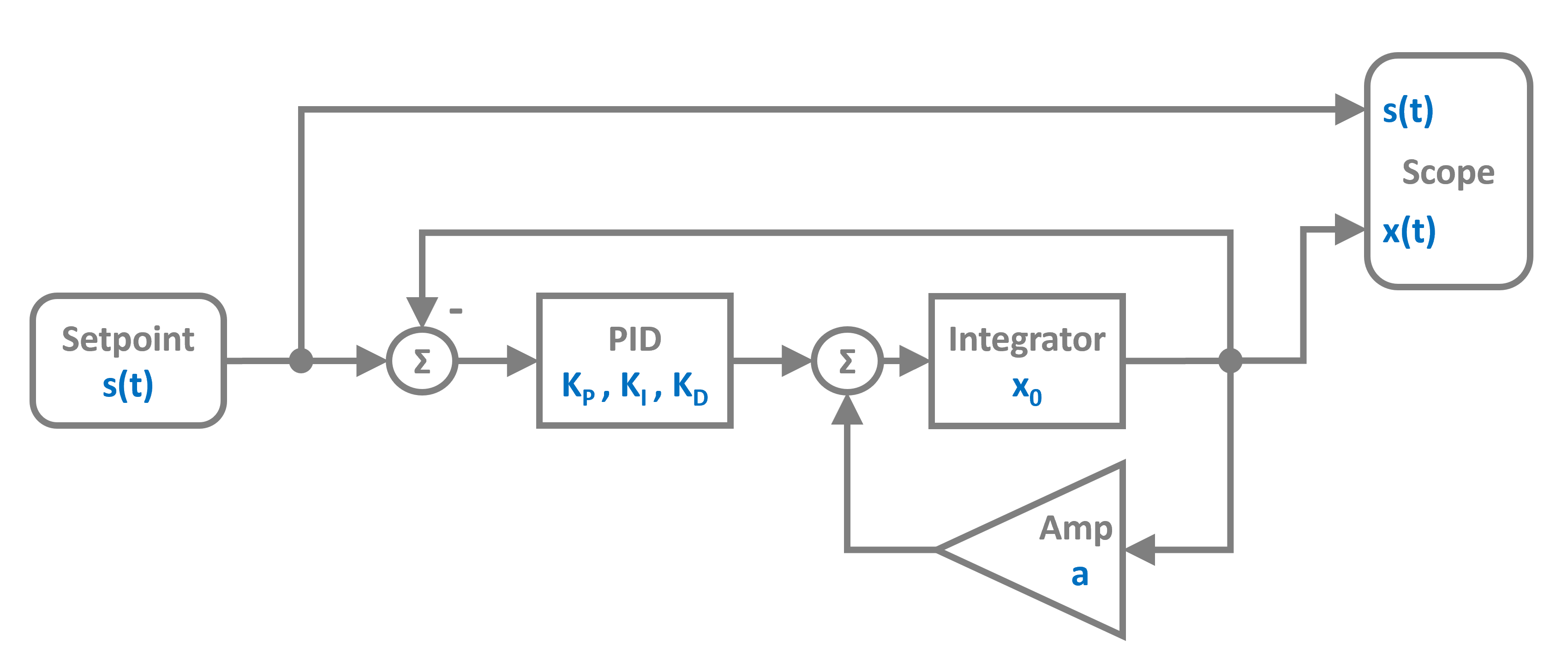
The control system uses a PID controller block that computes the control signal based on the error between setpoint and output. The plant is modeled as an Integrator with a gain. As a block diagram it looks like this:

Import and Setup

First let’s import the required classes and blocks:

import numpy as np
import matplotlib.pyplot as plt

# Apply PathSim docs matplotlib style
plt.style.use('../pathsim_docs.mplstyle')

from pathsim import Simulation, Connection
from pathsim.blocks import Source, Integrator, Amplifier, Adder, Scope, PID
from pathsim.solvers import RKCK54
from pathsim.optim import Value

System Parameters

We define the plant gain and PID parameters. Notice that we use Value to create the PID parameters - this enables automatic differentiation for sensitivity analysis.

# Plant gain
K = 0.4

# PID parameters (using Value for automatic differentiation)
Kp, Ki, Kd = Value.array([1.5, 0.5, 0.1])

# Setpoint function - step changes at t=20s and t=60s
def f_s(t):
    if t > 60:
        return 0.5
    elif t > 20:
        return 1
    else:
        return 0

System Definition

Now we can construct the system by instantiating the blocks we need and collecting them in a list:

# Blocks
spt = Source(f_s)
err = Adder("+-")  # Computes setpoint - output
pid = PID(Kp, Ki, Kd, f_max=10)  # PID with saturation
pnt = Integrator()
pgn = Amplifier(K)
sco = Scope(labels=["s(t)", "x(t)", r"$\epsilon(t)$"])

blocks = [spt, err, pid, pnt, pgn, sco]

The connections form a feedback control loop. The Adder block with signature "+-" computes the error signal by subtracting the plant output from the setpoint.

connections = [
    Connection(spt, err, sco[0]),      # Setpoint to error and scope
    Connection(pgn, err[1], sco[1]),   # Output to error (negative) and scope
    Connection(err, pid, sco[2]),      # Error to PID and scope
    Connection(pid, pnt),              # PID output to plant
    Connection(pnt, pgn)               # Plant to gain
]

Simulation Setup and Execution

We initialize the simulation with the RKCK54 solver (Runge-Kutta Cash-Karp 5th order with adaptive step size).

# Simulation initialization
Sim = Simulation(blocks, connections, Solver=RKCK54)

# Run the simulation for 100 seconds
Sim.run(100)

2025-10-23 15:25:45,477 - INFO - LOGGING (log: True)
2025-10-23 15:25:45,477 - INFO - BLOCK (type: Source, dynamic: False, events: 0)
2025-10-23 15:25:45,478 - INFO - BLOCK (type: Adder, dynamic: False, events: 0)
2025-10-23 15:25:45,478 - INFO - BLOCK (type: PID, dynamic: True, events: 0)
2025-10-23 15:25:45,479 - INFO - BLOCK (type: Integrator, dynamic: True, events: 0)
2025-10-23 15:25:45,479 - INFO - BLOCK (type: Amplifier, dynamic: False, events: 0)
2025-10-23 15:25:45,479 - INFO - BLOCK (type: Scope, dynamic: False, events: 0)
2025-10-23 15:25:45,481 - INFO - GRAPH (nodes: 6, edges: 8, alg. depth: 4, loop depth: 0, runtime: 0.062ms)
2025-10-23 15:25:45,481 - INFO - STARTING -> TRANSIENT (Duration: 100.00s)
2025-10-23 15:25:45,482 - INFO - TRANSIENT:   0% | elapsed: 00:00:00 (eta: --:--:--) | 0 steps (N/A steps/s)
2025-10-23 15:25:45,594 - INFO - TRANSIENT:  20% | elapsed: 00:00:00 (eta: 00:00:00) | 113 steps (1002.5 steps/s)
2025-10-23 15:25:45,680 - INFO - TRANSIENT:  40% | elapsed: 00:00:00 (eta: 00:00:00) | 198 steps (994.6 steps/s)
2025-10-23 15:25:45,816 - INFO - TRANSIENT:  60% | elapsed: 00:00:00 (eta: 00:00:00) | 335 steps (1008.1 steps/s)
2025-10-23 15:25:45,900 - INFO - TRANSIENT:  80% | elapsed: 00:00:00 (eta: 00:00:00) | 419 steps (995.5 steps/s)
2025-10-23 15:25:45,966 - INFO - TRANSIENT: 100% | elapsed: 00:00:00 (eta: 00:00:00) | 485 steps (995.9 steps/s)
2025-10-23 15:25:45,967 - INFO - TRANSIENT: 100% | elapsed: 00:00:00 (eta: 00:00:00) | 485 steps (998.7 avg steps/s)
2025-10-23 15:25:45,968 - INFO - FINISHED -> TRANSIENT (total steps: 485, successful: 316, runtime: 485.65 ms)

{'total_steps': 485, 'successful_steps': 316, 'runtime_ms': 485.64801500106114}

Results

Let’s plot the setpoint, output, and error signals to see how well the PID controller tracks the setpoint:

sco.plot(".-", lw=2)
plt.show()

Sensitivity Analysis

One of PathSim’s powerful features is automatic differentiation through the Value class. We can compute how sensitive the error signal is to each PID parameter using Value.der().

# Extract time and signals
time, [sp, ot, er] = sco.read()

# Plot sensitivities
fig, ax = plt.subplots(figsize=(8, 4), dpi=120, tight_layout=True)

ax.plot(time, Value.der(er, Kp), lw=2, label=r"$\partial \epsilon / \partial K_p $")
ax.plot(time, Value.der(er, Ki), lw=2, label=r"$\partial \epsilon / \partial K_i $")
ax.plot(time, Value.der(er, Kd), lw=2, label=r"$\partial \epsilon / \partial K_d $")

ax.legend(fancybox=False)
ax.set_xlabel("time [s]")
ax.set_ylabel("Sensitivity")
ax.grid()

plt.show()

The sensitivity plot shows which parameters most affect system performance. This information is useful for PID tuning and understanding the controller’s behavior.