Noisy Amplifier

The most simplistic model for an amplifier is just the product of a signal with some factor (gain). But we all know, real amplifiers are noisy and nonlinear. Internal physical processes or fluctiations in the power supply produce noise and if the amplitudes get too big, we run into saturations.

PathSim implements a number (WhiteNoiseSource and PinkNoiseSource) of broadband noise generators that produce accurate frequency domain noise spectra but for transient analysis.

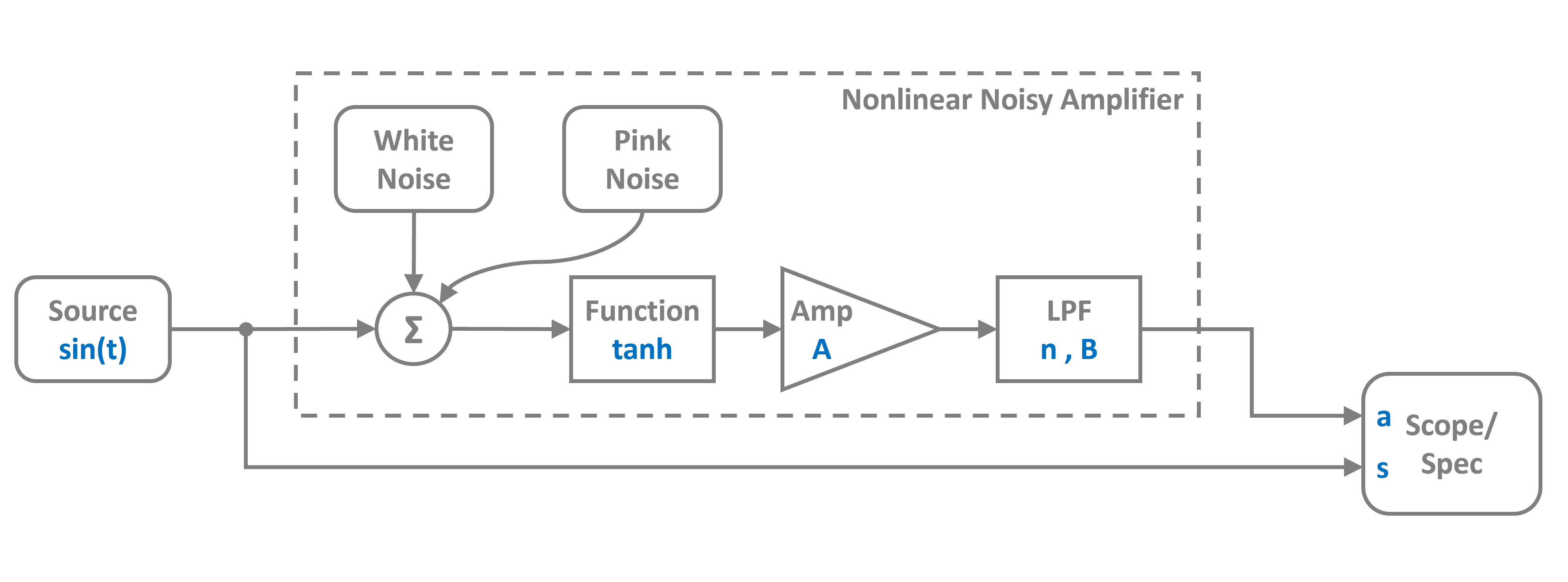
In this example we are bringing that together to implement a simple model of a nonlinear, noisy and band limited amplifier shown in the figure below:

import numpy as np
import matplotlib.pyplot as plt

# Apply PathSim docs matplotlib style
plt.style.use('../pathsim_docs.mplstyle')

from pathsim import Simulation, Connection, Subsystem, Interface

from pathsim.blocks import (
    Scope, Spectrum, Amplifier, Function, Adder, WhiteNoise,
    PinkNoise, SinusoidalSource, ButterworthLowpassFilter
    )

# For the automatic differentiation
from pathsim.optim import Value, der

Noisy Amplifier Model as Subsystem

The nonlinear amplifier model is defined as a Subsystem, implementing the gain as an elementary Amplifier block, the saturation (nonlinearity) as a Function block, wrapping a hyperbolic tangent and a ButterworthLowpassFilter for the frequency dependency. On top of that, two noise sources (WhiteNoiseSource and PinkNoiseSource) are added to the input of the model.

In addition to that we define the noise parameters as instances of the Value class. This enables the propagation of the partial derivatives with respect to these parameters through the whole simulation. And in the end we can do some cool noise sensitivity analysis and see how the noise spectrum is shaped through the nonlinearity and the filter. Note that using the Value class for simulation or model parameters massively slows down the simulation due to the overhead of gradient tracking.

# System parameters

a  = 10   # gain
fc = 1e6  # bandwidth
n  = 2    # filter order

# For sensitivity analysis
psd_w, psd_p = Value.array([1e-9, 1e-10])

# Internal subsystem blocks for the noisy amplifier

amp_int = Interface()
amp_wns = WhiteNoise(spectral_density=psd_w)
amp_pns = PinkNoise(spectral_density=psd_p)
amp_add = Adder()
amp_sat = Function(np.tanh)
amp_amp = Amplifier(a)
amp_flt = ButterworthLowpassFilter(fc, n)

amp_blocks = [amp_int, amp_wns, amp_pns, amp_add, amp_flt, amp_amp, amp_sat]

amp_connections = [
    Connection(amp_int, amp_add[0]),
    Connection(amp_wns, amp_add[1]),
    Connection(amp_pns, amp_add[2]),
    Connection(amp_add, amp_sat),
    Connection(amp_sat, amp_amp),
    Connection(amp_amp, amp_flt),
    Connection(amp_flt, amp_int)
    ]

AMP = Subsystem(amp_blocks, amp_connections)

Main System (Top Level)

The amplifier model is ready, we connect an sinusoidal source to its input and a spectrum analyzer (Spectrum) and Scope to its output.

Src = SinusoidalSource(frequency=2e5, amplitude=1)
Sco = Scope(labels=["Src", "AMP"])
Spc = Spectrum(freq=np.logspace(4.1, 7, 250), labels=["Src", "AMP"])

blocks = [AMP, Src, Sco, Spc]

connections = [
    Connection(Src, AMP, Sco[0], Spc[0]),
    Connection(AMP, Sco[1], Spc[1])
    ]

Sim = Simulation(
    blocks,
    connections,
    dt=3e-8,
    log=True
    )

2025-10-23 15:25:11,776 - INFO - LOGGING (log: True)
2025-10-23 15:25:11,777 - INFO - BLOCK (type: Subsystem, dynamic: True, events: 0)
2025-10-23 15:25:11,778 - INFO - BLOCK (type: SinusoidalSource, dynamic: False, events: 0)
2025-10-23 15:25:11,778 - INFO - BLOCK (type: Scope, dynamic: False, events: 0)
2025-10-23 15:25:11,778 - INFO - BLOCK (type: Spectrum, dynamic: True, events: 0)
2025-10-23 15:25:11,779 - INFO - GRAPH (nodes: 4, edges: 5, alg. depth: 1, loop depth: 0, runtime: 0.027ms)

Simulation

Lets run the simulation for some duration. Here 100us, 20 periods of the sinusoidal source.

Sim.run(1e-4);

2025-10-23 15:25:11,783 - INFO - STARTING -> TRANSIENT (Duration: 0.00s)
2025-10-23 15:25:11,784 - INFO - TRANSIENT:   0% | elapsed: 00:00:00 (eta: --:--:--) | 0 steps (N/A steps/s)
2025-10-23 15:25:12,786 - INFO - TRANSIENT:   4% | elapsed: 00:00:01 (eta: 00:00:24) | 130 steps (129.7 steps/s)
2025-10-23 15:25:13,792 - INFO - TRANSIENT:   8% | elapsed: 00:00:02 (eta: 00:00:23) | 260 steps (129.3 steps/s)
2025-10-23 15:25:14,799 - INFO - TRANSIENT:  12% | elapsed: 00:00:03 (eta: 00:00:22) | 400 steps (139.1 steps/s)
2025-10-23 15:25:15,800 - INFO - TRANSIENT:  16% | elapsed: 00:00:04 (eta: 00:00:21) | 529 steps (128.8 steps/s)
2025-10-23 15:25:16,805 - INFO - TRANSIENT:  20% | elapsed: 00:00:05 (eta: 00:00:20) | 658 steps (128.4 steps/s)
2025-10-23 15:25:16,870 - INFO - TRANSIENT:  20% | elapsed: 00:00:05 (eta: 00:00:20) | 667 steps (137.9 steps/s)
2025-10-23 15:25:17,875 - INFO - TRANSIENT:  24% | elapsed: 00:00:06 (eta: 00:00:19) | 797 steps (129.5 steps/s)
2025-10-23 15:25:18,910 - INFO - TRANSIENT:  28% | elapsed: 00:00:07 (eta: 00:00:18) | 931 steps (129.4 steps/s)
2025-10-23 15:25:19,911 - INFO - TRANSIENT:  32% | elapsed: 00:00:08 (eta: 00:00:17) | 1070 steps (138.9 steps/s)
2025-10-23 15:25:20,914 - INFO - TRANSIENT:  36% | elapsed: 00:00:09 (eta: 00:00:16) | 1198 steps (127.6 steps/s)
2025-10-23 15:25:21,919 - INFO - TRANSIENT:  40% | elapsed: 00:00:10 (eta: 00:00:15) | 1326 steps (127.3 steps/s)
2025-10-23 15:25:21,978 - INFO - TRANSIENT:  40% | elapsed: 00:00:10 (eta: 00:00:15) | 1334 steps (137.1 steps/s)
2025-10-23 15:25:22,978 - INFO - TRANSIENT:  44% | elapsed: 00:00:11 (eta: 00:00:14) | 1461 steps (126.9 steps/s)
2025-10-23 15:25:23,984 - INFO - TRANSIENT:  48% | elapsed: 00:00:12 (eta: 00:00:13) | 1601 steps (139.1 steps/s)
2025-10-23 15:25:24,991 - INFO - TRANSIENT:  52% | elapsed: 00:00:13 (eta: 00:00:12) | 1731 steps (129.1 steps/s)
2025-10-23 15:25:25,996 - INFO - TRANSIENT:  56% | elapsed: 00:00:14 (eta: 00:00:11) | 1860 steps (128.3 steps/s)
2025-10-23 15:25:27,000 - INFO - TRANSIENT:  60% | elapsed: 00:00:15 (eta: 00:00:10) | 1989 steps (128.5 steps/s)
2025-10-23 15:25:27,088 - INFO - TRANSIENT:  60% | elapsed: 00:00:15 (eta: 00:00:10) | 2001 steps (137.4 steps/s)
2025-10-23 15:25:28,089 - INFO - TRANSIENT:  64% | elapsed: 00:00:16 (eta: 00:00:09) | 2140 steps (138.8 steps/s)
2025-10-23 15:25:29,091 - INFO - TRANSIENT:  68% | elapsed: 00:00:17 (eta: 00:00:08) | 2268 steps (127.7 steps/s)
2025-10-23 15:25:30,098 - INFO - TRANSIENT:  72% | elapsed: 00:00:18 (eta: 00:00:07) | 2398 steps (129.1 steps/s)
2025-10-23 15:25:31,100 - INFO - TRANSIENT:  76% | elapsed: 00:00:19 (eta: 00:00:06) | 2526 steps (127.9 steps/s)
2025-10-23 15:25:32,100 - INFO - TRANSIENT:  80% | elapsed: 00:00:20 (eta: 00:00:05) | 2665 steps (138.9 steps/s)
2025-10-23 15:25:32,115 - INFO - TRANSIENT:  80% | elapsed: 00:00:20 (eta: 00:00:05) | 2667 steps (130.3 steps/s)
2025-10-23 15:25:33,118 - INFO - TRANSIENT:  84% | elapsed: 00:00:21 (eta: 00:00:04) | 2796 steps (128.7 steps/s)
2025-10-23 15:25:34,121 - INFO - TRANSIENT:  88% | elapsed: 00:00:22 (eta: 00:00:03) | 2925 steps (128.5 steps/s)
2025-10-23 15:25:35,135 - INFO - TRANSIENT:  92% | elapsed: 00:00:23 (eta: 00:00:02) | 3055 steps (128.2 steps/s)
2025-10-23 15:25:36,141 - INFO - TRANSIENT:  96% | elapsed: 00:00:24 (eta: 00:00:01) | 3194 steps (138.2 steps/s)
2025-10-23 15:25:37,143 - INFO - TRANSIENT: 100% | elapsed: 00:00:25 (eta: 00:00:00) | 3322 steps (127.7 steps/s)
2025-10-23 15:25:37,231 - INFO - TRANSIENT: 100% | elapsed: 00:00:25 (eta: 00:00:00) | 3334 steps (137.0 steps/s)
2025-10-23 15:25:37,232 - INFO - TRANSIENT: 100% | elapsed: 00:00:25 (eta: 00:00:00) | 3334 steps (131.0 avg steps/s)
2025-10-23 15:25:37,232 - INFO - FINISHED -> TRANSIENT (total steps: 3334, successful: 3334, runtime: 25448.52 ms)

Results

We can read the time series results and see that we get the expected amplified sinusoid. The noise parameters we chose are pretty big, so we can see the fluctuations.

time, [res_src, res_amp] = Sco.read()

fig, ax = plt.subplots(nrows=1, figsize=(8, 4), tight_layout=True, dpi=200)

ax.plot(time, res_src, label=Sco.labels[0])
ax.plot(time, res_amp, label=Sco.labels[1])
ax.set_xlabel("time [s]")
ax.legend();

In the frequency domain we can see the second peak in te spectrum of the output signal. This indicates the nonlinearity.

freq, [res_src, res_amp] = Spc.read()

fig, ax = plt.subplots(figsize=(8, 4), tight_layout=True, dpi=200)

ax.loglog(freq, abs(res_src), label=Spc.labels[0])
ax.loglog(freq, abs(res_amp), label=Spc.labels[1])

ax.set_xlabel("Freq [Hz]")
ax.set_ylabel("Magnitude")
ax.set_ylim(1e-6, None)
ax.legend();

Sensitivity Analysis

Now comes the fun part. We can extract the partial derivatives with respect to the noise parameters directly from the simulation results. The gradients are tracked through the whole simulation thanks to the automatic differentiation, the Value class provides.

# time domain sensitivities

time, [res_src, res_amp] = Sco.read()

# extract partial derivatives
d_res_amp_d_psd_w = der(res_amp, psd_w)
d_res_amp_d_psd_p = der(res_amp, psd_p)

fig, ax = plt.subplots(nrows=1, figsize=(8, 4), tight_layout=True, dpi=200)

ax.plot(time, psd_w*d_res_amp_d_psd_w,
    label=r"$\mathrm{psd}_w \dfrac{\partial \mathrm{AMP}}{\partial \mathrm{psd}_w}$")
ax.plot(time, psd_p*d_res_amp_d_psd_p,
    label=r"$\mathrm{psd}_p \dfrac{\partial \mathrm{AMP}}{\partial \mathrm{psd}_p}$")

ax.set_xlabel("time [s]")
ax.legend();

The same holds for the spectrum that the Spectrum block computes. The Value instances propagate even through the internal running fourier transform (RFT) and the partial derivatives of the complex spectrum can just be extracted from the result.

We can clearly see the nearly undisturbed white and pink noise spectra at low frequencies and the effect of the low pass filter at the higher frequencies.

# spectral sensitivities

freq, [res_src, res_amp] = Spc.read()

# extract partial derivatives
d_res_amp_d_psd_w = der(res_amp, psd_w)
d_res_amp_d_psd_p = der(res_amp, psd_p)

fig, ax = plt.subplots(figsize=(8, 4), tight_layout=True, dpi=200)

ax.loglog(freq, abs(psd_w*d_res_amp_d_psd_w),
    label=r"$\mathrm{psd}_w \dfrac{\partial \mathrm{AMP}}{\partial \mathrm{psd}_w}$")
ax.loglog(freq, abs(psd_p*d_res_amp_d_psd_p),
    label=r"$\mathrm{psd}_p \dfrac{\partial \mathrm{AMP}}{\partial \mathrm{psd}_p}$")
ax.set_xlabel("freq [Hz]")
ax.legend(ncol=2);