Delta-Sigma ADC

You can also find this example as a single file in the GitHub repository.This example demonstrates a first-order delta-sigma (ΔΣ) ADC, a popular architecture for high-resolution analog-to-digital conversion. The system uses oversampling and noise shaping to achieve high precision with a simple 1-bit quantizer.

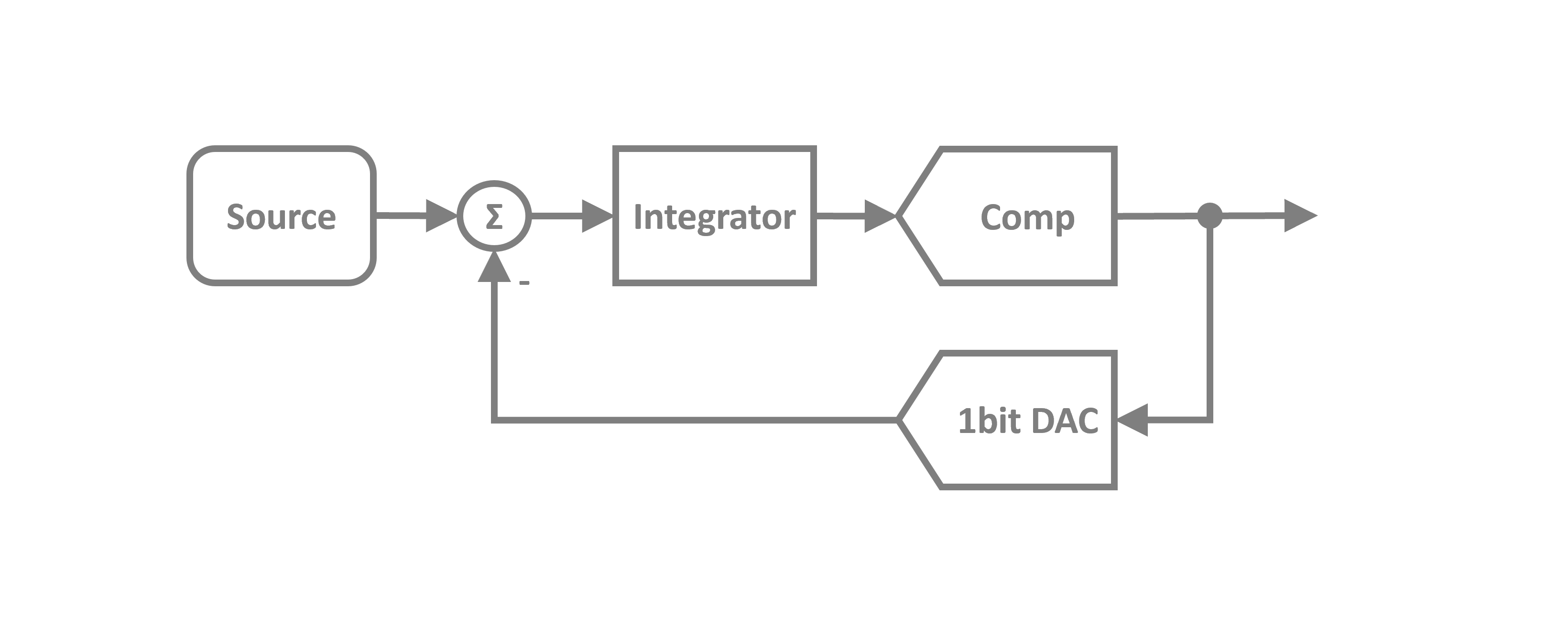
Delta-Sigma ADC Principle

A delta-sigma ADC works by:

1. Oversampling the input signal at a high frequency

2. Using a 1-bit quantizer (comparator)

3. Negative feedback through a DAC to shape quantization noise

4. Digital filtering (FIR) to downsample and reconstruct the signal

The key advantage is that quantization noise is pushed to high frequencies (noise shaping), where it can be filtered out.

The system uses DAC, Comparator, SampleHold, and FIR blocks to implement a complete delta-sigma ADC with digital filtering.

import numpy as np
import matplotlib.pyplot as plt
from scipy.signal import firwin

# Apply PathSim docs matplotlib style for consistent, theme-friendly figures
plt.style.use('../pathsim_docs.mplstyle')

from pathsim import Simulation, Connection
from pathsim.blocks import (
    Integrator, Adder, Scope, Source,
    SampleHold, DAC, Comparator, FIR
)
from pathsim.solvers import RKBS32

System Parameters

We set the key parameters:

• Clock frequency: 100 Hz (oversampling rate)

• Reference voltage: 1.0 V

• FIR filter: 20 taps, cutoff at Fs/50

The input signal is a 1 Hz sine wave, so the oversampling ratio is 100.

v_ref = 1.0           # DAC reference
f_clk = 100           # Sampling frequency
T_clk = 1.0 / f_clk   # Sampling period

# Design FIR lowpass filter for decimation
fir_coeffs = firwin(20, f_clk/50, fs=f_clk)

Block Diagram

We create the blocks for the delta-sigma modulator:

• src: Input signal (sine wave)

• sub: Subtractor (input - feedback)

• itg: Integrator (loop filter)

• sah: Sample & Hold

• qtz: Comparator (1-bit quantizer)

• dac: 1-bit DAC for feedback

• lpf: FIR lowpass filter for reconstruction

# Blocks that define the system
src = Source(lambda t: np.sin(2*np.pi*t))
sub = Adder("+-")
itg = Integrator()
sah = SampleHold(T=T_clk, tau=T_clk*1e-3)
qtz = Comparator(span=[0, 1])
dac = DAC(n_bits=1, span=[-v_ref, v_ref], T=T_clk, tau=T_clk*2e-3)
lpf = FIR(coeffs=fir_coeffs, T=T_clk, tau=T_clk*2e-3)
sc1 = Scope(labels=["src", "qtz", "dac", "lpf"])
sc2 = Scope(labels=["itg", "sah"])

blocks = [src, sub, itg, sah, qtz, dac, lpf, sc1, sc2]

Connections

The connections form the delta-sigma loop with digital filtering.

connections = [
    Connection(src, sub[0], sc1[0]),      # Source to subtractor and scope
    Connection(dac, sub[1], lpf, sc1[2]), # DAC feedback and to FIR filter
    Connection(sub, itg),                 # Difference to integrator
    Connection(itg, sah, sc2[0]),         # Integrator to S&H
    Connection(sah, qtz, sc2[1]),         # S&H to comparator
    Connection(qtz, dac[0], sc1[1]),      # Comparator to DAC
    Connection(lpf, sc1[3]),              # Filtered output
]

Simulation

We use an adaptive solver (RKBS32) with a maximum timestep to handle the discrete-time sampling events properly.

# Simulation with adaptive solver
Sim = Simulation(
    blocks,
    connections,
    dt_max=T_clk*0.1,
    Solver=RKBS32
)

# Run simulation for 2 seconds
Sim.run(2)

2025-10-23 15:24:23,549 - INFO - LOGGING (log: True)
2025-10-23 15:24:23,550 - INFO - BLOCK (type: Source, dynamic: False, events: 0)
2025-10-23 15:24:23,551 - INFO - BLOCK (type: Adder, dynamic: False, events: 0)
2025-10-23 15:24:23,551 - INFO - BLOCK (type: Integrator, dynamic: True, events: 0)
2025-10-23 15:24:23,552 - INFO - BLOCK (type: SampleHold, dynamic: False, events: 1)
2025-10-23 15:24:23,552 - INFO - BLOCK (type: Comparator, dynamic: False, events: 1)
2025-10-23 15:24:23,552 - INFO - BLOCK (type: DAC, dynamic: False, events: 1)
2025-10-23 15:24:23,552 - INFO - BLOCK (type: FIR, dynamic: False, events: 1)
2025-10-23 15:24:23,553 - INFO - BLOCK (type: Scope, dynamic: False, events: 0)
2025-10-23 15:24:23,553 - INFO - BLOCK (type: Scope, dynamic: False, events: 0)
2025-10-23 15:24:23,555 - INFO - GRAPH (nodes: 9, edges: 13, alg. depth: 2, loop depth: 0, runtime: 0.060ms)
2025-10-23 15:24:23,555 - INFO - STARTING -> TRANSIENT (Duration: 2.00s)
2025-10-23 15:24:23,556 - INFO - TRANSIENT:   0% | elapsed: 00:00:00 (eta: --:--:--) | 0 steps (N/A steps/s)
2025-10-23 15:24:23,637 - INFO - TRANSIENT:  20% | elapsed: 00:00:00 (eta: --:--:--) | 482 steps (5900.3 steps/s)
2025-10-23 15:24:23,719 - INFO - TRANSIENT:  40% | elapsed: 00:00:00 (eta: 00:00:00) | 962 steps (5873.4 steps/s)
2025-10-23 15:24:23,800 - INFO - TRANSIENT:  60% | elapsed: 00:00:00 (eta: 00:00:00) | 1442 steps (5895.1 steps/s)
2025-10-23 15:24:23,883 - INFO - TRANSIENT:  80% | elapsed: 00:00:00 (eta: 00:00:00) | 1922 steps (5818.0 steps/s)
2025-10-23 15:24:23,965 - INFO - TRANSIENT: 100% | elapsed: 00:00:00 (eta: 00:00:00) | 2402 steps (5836.2 steps/s)
2025-10-23 15:24:23,967 - INFO - TRANSIENT: 100% | elapsed: 00:00:00 (eta: 00:00:00) | 2402 steps (5836.6 avg steps/s)
2025-10-23 15:24:23,967 - INFO - FINISHED -> TRANSIENT (total steps: 2402, successful: 2401, runtime: 411.54 ms)

{'total_steps': 2402,
 'successful_steps': 2401,
 'runtime_ms': 411.5426809985365}

Results

The plots show:

1. src (blue): Original analog input signal

2. qtz (orange): 1-bit quantizer output (high-frequency switching)

3. dac (green): 1-bit DAC feedback signal

4. lpf (red): Reconstructed signal after FIR filtering

Notice how the 1-bit stream encodes the analog signal, and the FIR filter successfully reconstructs it.

Sim.plot()
plt.show()