Harmonic Oscillator
In this example we have a look at the damped harmonic oscillator. A linear dynamical system that models a spring-mass-damper system.
You can also find this example as a single file in the GitHub repository.
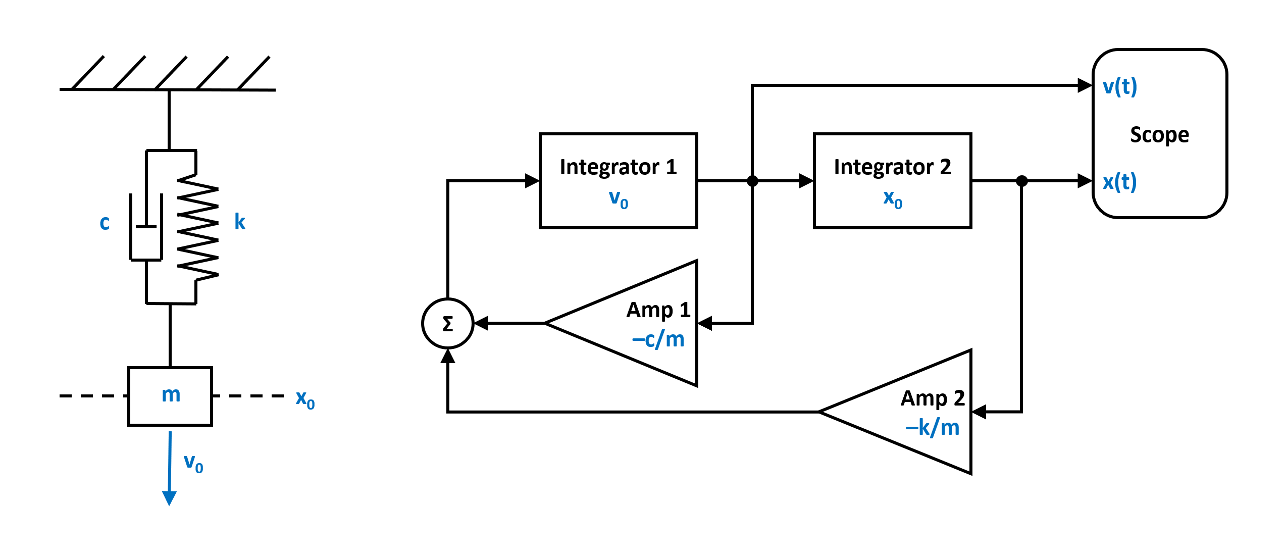
The equation of motion that defines the harmonic oscillator it is given by
where c is the damping, k the spring constant (stiffness) and m the mass. The corresponding block diagramm can be translated into a netlist by using the blocks and the connection class provided by PathSim.
First lets import the Simulation and Connection classes and the required blocks from the block library:
from pathsim import Simulation, Connection
from pathsim.blocks import Integrator, Amplifier, Adder, Scope
Then lets define the system parameters:
#initial position and velocity
x0, v0 = 2, 5

#parameters (mass, damping, spring constant)
m, c, k = 0.8, 0.2, 1.5
Now we can construct the system by instantiating the blocks we need (from the block diagram above) with their corresponding prameters and collect them together in a list:
#blocks that define the system
I1 = Integrator(v0)   # integrator for velocity
I2 = Integrator(x0)   # integrator for position
A1 = Amplifier(c)
A2 = Amplifier(k)
A3 = Amplifier(-1/m)
P1 = Adder()
Sc = Scope(labels=["velocity", "position"])

blocks = [I1, I2, A1, A2, A3, P1, Sc]
Afterwards, the connections between the blocks can be defined. The first argument of the Connection class is the source block and its port (Sc[1] would be port 1 of the instance of the Scope block).
#the connections between the blocks
connections = [
    Connection(I1, I2, A1, Sc),
    Connection(I2, A2, Sc[1]),
    Connection(A1, P1),
    Connection(A2, P1[1]),
    Connection(P1, A3),
    Connection(A3, I1)
    ]
Finally we can instantiate the Simulation with the blocks, connections and some additional parameters such as the timestep. In this case, no special ODE solver is specified, so PathSim uses the default SSPRK22 integrator which is a fixed step 2nd order explicit Runge-Kutta method. A good starting point for non stiff linear systems like this.
#initialize simulation with the blocks, connections, timestep
Sim = Simulation(blocks, connections, dt=0.01, log=True)
Then we can run the simulation for some duration:
#run the simulation for 20 seconds
Sim.run(duration=25)
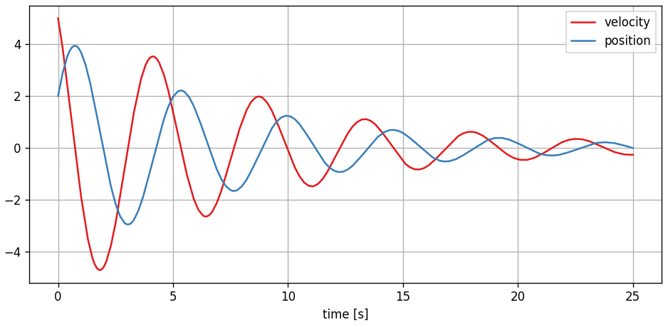
Due to the object oriented and decentralized nature of PathSim, the Scope block holds the recorded time series data from the simulation internally. It can be plotted directly in an external matplotlib window using the plot method
#plot the results from the scope
Sc.plot()
which looks like an exponentially decaying sinusoid: