Van der Pol¶

Simulation of the Van der Pol oscillator, a classic example of a stiff dynamical system.

You can also find this example as a single file in the GitHub repository.

The Van der Pol oscillator is described by the following 2nd order ODE

\[\ddot{x} + \mu (x^2 - 1) \dot{x} + x = 0\]

where the parameter \(\mu\) controles the stiffness of the system. Stiffness in dynamical systems typically arises when the (local) internal time constants (eigenvalues of the Jacobian) are on different scales, or when very steep gradients are encountered.

ODE solvers for stiff systems require large stability regions and therefore are usually implicit. PathSim has a huge range of implicit solvers (i.e. ESDIRK32, ESDIRK43, GEAR52A, …), that can be used to solve stiff systems, such as the Van der Pol system with very large \(\mu\), reliably. Lets see how this works.

PathSim supplies a specific block to define differential equations, the ODE block. To accept the Van der Pol system, we have to convert the 2nd order ODE into a system of 1st order ODEs:

\[\begin{split}\begin{align} \dot{x}_1 &= x_2 \\ \dot{x}_2 &= \mu (1 - x_1^2) x_2 - x_1 \end{align}\end{split}\]

As a block diagram it would look like this:

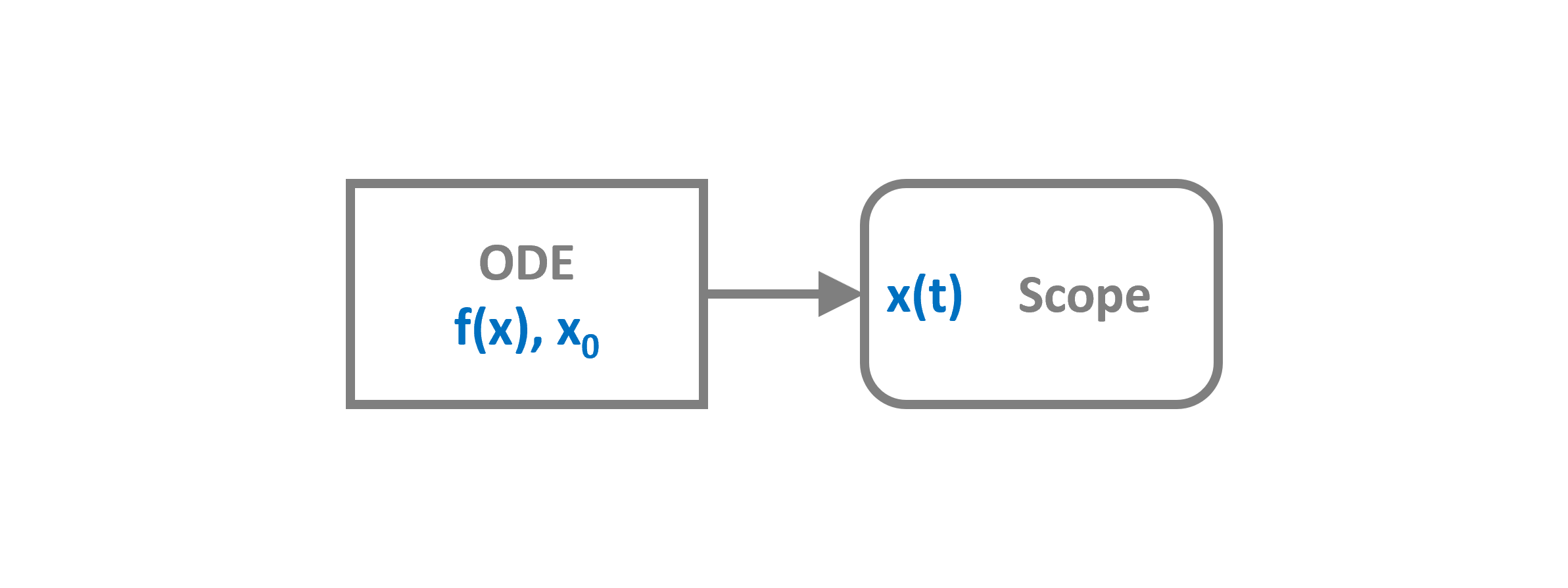
And translated to PathSim like this:

[1]:

import numpy as np
import matplotlib.pyplot as plt

# Apply PathSim docs matplotlib style for consistent, theme-friendly figures
plt.style.use('../pathsim_docs.mplstyle')

from pathsim import Simulation, Connection
from pathsim.blocks import Scope, ODE
from pathsim.solvers import GEAR52A # <- implicit solver for stiff systems

# Initial condition
x0 = np.array([2, 0])

# Van der Pol parameter
mu = 1000 # <- this is very stiff

def func(x, u, t):
    return np.array([x[1], mu*(1 - x[0]**2)*x[1] - x[0]])

# Analytical jacobian (optional)
def jac(x, u, t):
    return np.array([[0, 1], [-mu*2*x[0]*x[1]-1, mu*(1 - x[0]**2)]])

# Blocks that define the system
VDP = ODE(func, x0, jac) # jacobian improves convergence
Sco = Scope(labels=[r"$x_1(t)$"])

blocks = [VDP, Sco]

# The connect the blocks
connections = [
    Connection(VDP, Sco)
]

# Initialize simulation
Sim = Simulation(
    blocks,
    connections,
    Solver=GEAR52A,
    tolerance_lte_abs=1e-5,
    tolerance_lte_rel=1e-3,
    tolerance_fpi=1e-8
)

12:58:44 - INFO - LOGGING (log: True)
12:58:44 - INFO - BLOCKS (total: 2, dynamic: 1, static: 1, eventful: 0)
12:58:44 - INFO - GRAPH (nodes: 2, edges: 1, alg. depth: 1, loop depth: 0, runtime: 0.029ms)

Here we define the paramter \(\mu = 1000\) (btw. \(\mu = 10000\) also works), which means severe stiffness! This is pretty much a torture test for stiff ODE solvers.

Lets run the simulation and look at the results:

[2]:

# Run it
Sim.run(4*mu)

# Plotting
fig, ax = Sco.plot(".-")
plt.show()

12:58:44 - INFO - STARTING -> TRANSIENT (Duration: 4000.00s)
12:58:44 - INFO - --------------------   2% | 0.0s<0.1s | 1078.6 it/s
12:58:44 - INFO - ####----------------  20% | 0.1s<9.6s | 756.5 it/s
12:58:44 - INFO - ########------------  40% | 0.4s<2.8s | 673.6 it/s
12:58:44 - INFO - ############--------  60% | 0.7s<0.5s | 649.2 it/s
12:58:45 - INFO - ################----  80% | 1.0s<0.2s | 636.0 it/s
12:58:45 - INFO - #################### 100% | 1.3s<--:-- | 686.4 it/s
12:58:45 - INFO - FINISHED -> TRANSIENT (total steps: 817, successful: 567, runtime: 1289.70 ms)