SAR ADC

Simulation of a Successive Approximation Register ADC with custom block creation.

You can also find this example as a single file in the GitHub repository.

Successive Approximation Register (SAR) ADC Principle

A SAR ADC converts analog signals to digital using a binary search algorithm:

1. Sample the input voltage

2. Test the MSB (Most Significant Bit) by comparing to DAC output

3. Keep the bit if comparison succeeds, discard if it fails

4. Repeat for each bit from MSB to LSB

5. Output the complete digital word

This requires N comparisons for N bits, making it efficient for medium-speed, medium-resolution applications (10-18 bits, up to several MHz).

Custom SAR Logic Block

We’ll implement the SAR control logic as a custom block using PathSim’s event system.

This example shows how to create custom blocks by extending the Block class and using Schedule events for discrete-time logic.

import numpy as np
import matplotlib.pyplot as plt

# Apply PathSim docs matplotlib style for consistent, theme-friendly figures
plt.style.use('../pathsim_docs.mplstyle')

from pathsim import Simulation, Connection
from pathsim.blocks import (
    Adder, Scope, Source, ButterworthLowpassFilter,
    SampleHold, Comparator, DAC
)
from pathsim.solvers import RKBS32

Creating a Custom SAR Logic Block

This is one of PathSim’s powerful features - you can create custom blocks with complex behavior. The SAR block:

• Uses scheduled events to step through bits

• Implements the binary search algorithm

• Outputs N parallel digital signals (one per bit)

from pathsim.blocks._block import Block
from pathsim.utils.register import Register
from pathsim.events import Schedule

class SAR(Block):
    """Successive Approximation Register Logic

    Implements SAR algorithm for ADC conversion:
    - Reads comparator result
    - Updates trial bit pattern
    - Outputs N-bit digital word
    """

    def __init__(self, n_bits=4, T=1, tau=0):
        super().__init__()

        self.n_bits = n_bits
        self.T = T
        self.tau = tau

        self.register = 0
        self.trial_weight = 1 << (self.n_bits - 1)  # Start with MSB

        self.outputs = Register(self.n_bits)

        def _step(t):
            """SAR algorithm step - executes at each clock cycle"""
            comparator_result = self.inputs[0]

            previous_weight = (self.trial_weight << 1) if self.trial_weight > 0 else 1

            # If previous comparison failed, clear that bit
            if previous_weight <= (1 << (self.n_bits -1)) and comparator_result == 0:
                self.register &= ~previous_weight

            # Set current trial bit
            self.register |= self.trial_weight

            # Update all output bits
            for i in range(self.n_bits):
                self.outputs[i] = (self.register >> i) & 1

            # Move to next bit or restart
            if self.trial_weight == 1:
                self.trial_weight = 1 << (self.n_bits - 1)
                self.register = 0
            else:
                self.trial_weight >>= 1

        # Schedule event for SAR stepping
        self.events = [
            Schedule(
                t_start=self.tau,
                t_period=self.T/self.n_bits,  # One step per bit
                func_act=_step
            )
        ]

    def __len__(self):
        return 0

System Parameters

We’ll use:

• 8-bit resolution

• 50 Hz sampling frequency

• Modulated sine wave as input signal

n = 8                 # Number of bits
f_clk = 50            # Sampling frequency
T_clk = 1.0 / f_clk   # Sampling period

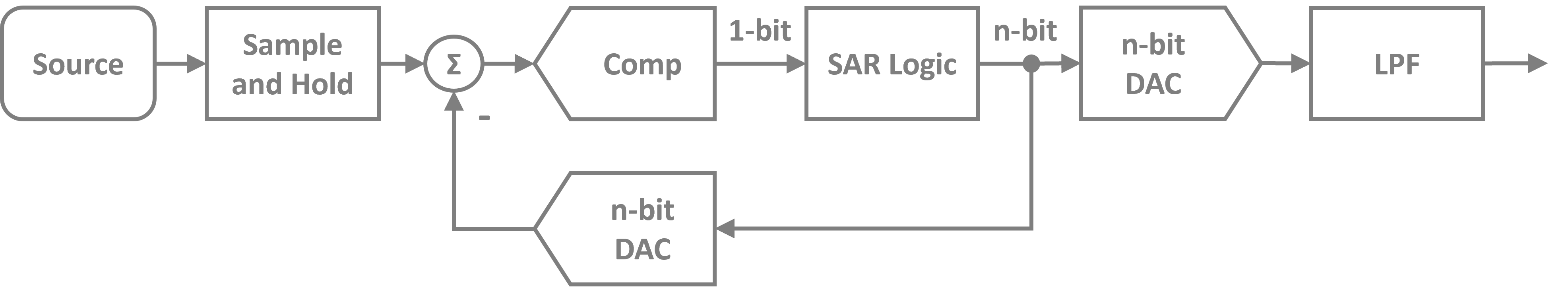
Block Diagram Setup

The system consists of:

• src: Modulated sine wave source

• sah: Sample & Hold to freeze input during conversion

• sub: Subtractor (input - DAC)

• cpt: Comparator

• sar: Custom SAR logic

• dac1: Fast DAC for comparison (updates every bit)

• dac2: Output DAC (updates every sample)

• lpf: Lowpass filter for reconstruction

# Blocks that define the system
src = Source(lambda t: np.sin(2*np.pi*t) * np.cos(5*np.pi*t))
sah = SampleHold(T=T_clk)
sub = Adder("+-")
cpt = Comparator(span=[0, 1])
dac1 = DAC(n_bits=n, T=T_clk/n, tau=T_clk*2e-3)  # Fast DAC for comparison
dac2 = DAC(n_bits=n, T=T_clk, tau=T_clk)         # Output DAC
lpf = ButterworthLowpassFilter(f_clk/5, n=3)     # Reconstruction filter
sar = SAR(n_bits=n, T=T_clk, tau=T_clk*1e-3)
sco = Scope(labels=["src", "sah", "dac1", "dac2", "lpf"])

blocks = [src, cpt, dac1, dac2, lpf, sar, sah, sub, sco]

Connections

The connections form the SAR ADC loop. Notice how the 8 digital bits from SAR connect to both DACs in parallel.

# Connections between the blocks
connections = [
    Connection(src, sah, sco[0]),        # Source to S&H and scope
    Connection(sah, sub[0], sco[1]),     # S&H to subtractor
    Connection(dac1, sub[1], sco[2]),    # DAC1 feedback to subtractor
    Connection(dac2, lpf, sco[3]),       # DAC2 to filter
    Connection(lpf, sco[4]),             # Filtered output
    Connection(sub, cpt),                # Difference to comparator
    Connection(cpt, sar)                 # Comparator to SAR logic
]

# Connect all N bits from SAR to both DACs
for i in range(n):
    connections.append(
        Connection(sar[i], dac1[i], dac2[i])
    )

Simulation

We run the simulation with an adaptive solver that can handle the discrete-time events efficiently.

# Simulation with adaptive solver
Sim = Simulation(
    blocks,
    connections,
    Solver=RKBS32
)

# Run simulation for 1 second
Sim.run(1)

12:58:17 - INFO - LOGGING (log: True)
12:58:17 - INFO - BLOCKS (total: 9, dynamic: 1, static: 8, eventful: 5)
12:58:17 - INFO - GRAPH (nodes: 9, edges: 27, alg. depth: 3, loop depth: 0, runtime: 0.169ms)
12:58:17 - INFO - STARTING -> TRANSIENT (Duration: 1.00s)
12:58:17 - INFO - --------------------   1% | 0.0s<0.5s | 2713.5 it/s
12:58:18 - INFO - ####----------------  20% | 0.2s<0.8s | 2762.6 it/s
12:58:18 - INFO - ########------------  40% | 0.3s<0.3s | 2717.0 it/s
12:58:18 - INFO - ############--------  60% | 0.5s<0.3s | 2736.2 it/s
12:58:18 - INFO - ################----  80% | 0.6s<0.1s | 2692.8 it/s
12:58:18 - INFO - #################### 100% | 0.8s<--:-- | 2640.7 it/s
12:58:18 - INFO - FINISHED -> TRANSIENT (total steps: 2124, successful: 2034, runtime: 779.80 ms)

{'total_steps': 2124,
 'successful_steps': 2034,
 'runtime_ms': 779.7950820095139}

Results

The plots show:

• src: Original analog input

• sah: Sampled and held signal

• dac1: Fast DAC during conversion (shows binary search)

• dac2: Output DAC (quantized signal)

• lpf: Reconstructed signal after filtering

Notice how dac1 shows the successive approximation steps within each sample period!

Sim.plot()
plt.show()