Billards & Collisions

You can also find this example as a standalone Python file in the GitHub repository.

This example demonstrates how to simulate a ball bouncing inside a circular boundary using PathSim’s event detection system. The ball is subject to gravity and bounces elastically off the circular wall. This showcases the use of zero-crossing events to detect and handle collisions.

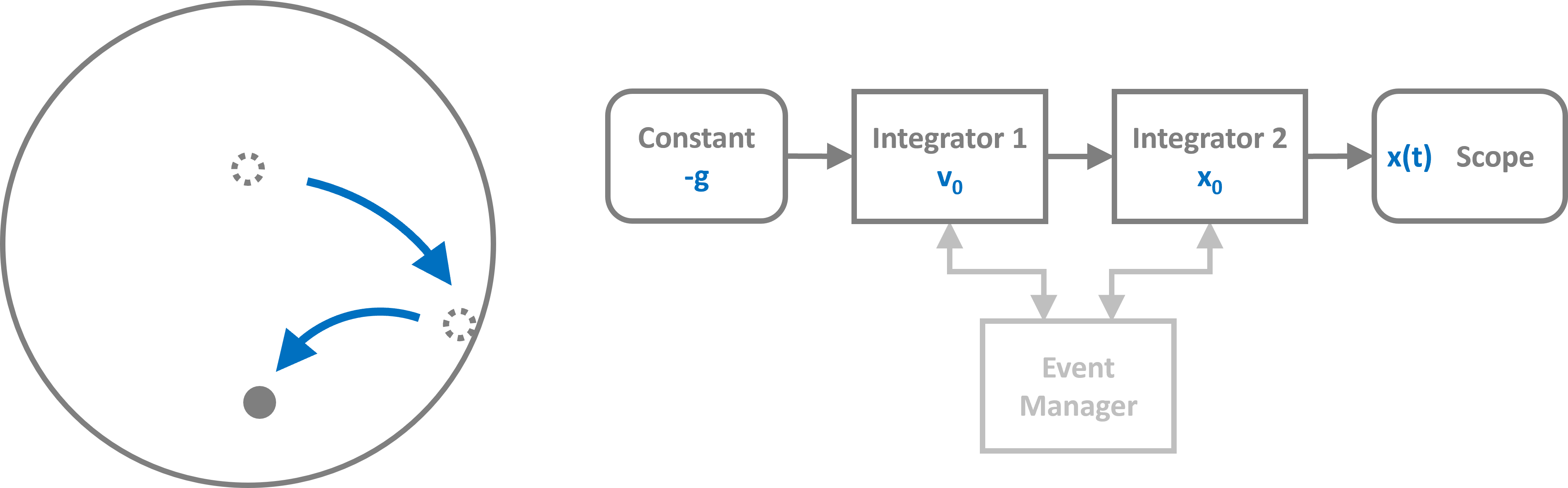
The physics of this system involves a point mass moving under gravity inside a circular container of radius \(l\). When the ball reaches the boundary, it reflects elastically. The reflection is computed by projecting the velocity onto the normal vector at the collision point and reversing that component.

import numpy as np
import matplotlib.pyplot as plt

# Apply PathSim docs matplotlib style
plt.style.use('../pathsim_docs.mplstyle')

from pathsim import Simulation, Connection
from pathsim.blocks import Constant, Integrator, Scope
from pathsim.events import ZeroCrossingUp
from pathsim.solvers import RKBS32

We define the system parameters: gravity \(g\), the radius \(l\) of the circular boundary, and the initial position and velocity of the ball.

# System parameters
g = 9.81   # gravity [m/s^2]
l = 1      # radius of circular boundary [m]

# Initial conditions
x0 = np.array([0.5, 0.5])  # initial position [m]
v0 = np.array([0, 0])      # initial velocity [m/s]

The dynamics are modeled using two Integrator blocks: one for position and one for velocity. A Constant block provides the gravitational acceleration acting on the y-component of velocity. The Scope block records the position for visualization.

# Blocks for dynamics
cn = Constant(-g)                    # gravitational acceleration
ix = Integrator(x0)                  # position integrator
iv = Integrator(v0)                  # velocity integrator
sc = Scope(labels=["x", "y"])        # scope to record position

Collision Detection and Response

The collision is detected using a zero-crossing event. The detection function computes the distance from the origin minus the boundary radius:

\[f(x) = \|x\| - l\]

When this function crosses zero from below (the ball reaches the boundary), the action function is triggered. The elastic reflection is computed as:

\[v_{\text{new}} = v - 2(v \cdot n)n\]

where \(n = x / \|x\|\) is the outward normal at the collision point.

# Collision event functions
def bounce_detect(_):
    """Detect when ball reaches boundary."""
    x = ix.engine.get()
    return np.linalg.norm(x) - l

def bounce_act(_):
    """Reflect velocity elastically off boundary."""
    v = iv.engine.get()
    x = ix.engine.get()
    n = x / np.linalg.norm(x)  # outward normal
    iv.engine.set(v - 2 * np.dot(v, n) * n)  # reflect velocity
    ix.engine.set(l * n)  # ensure position is exactly on boundary

Now we assemble the Simulation with all blocks, connections, and events. The gravity acts only on the y-component of velocity (channel 1). Both position components are connected to the scope for recording.

# Simulation definition
sim = Simulation(
    blocks=[ix, iv, sc, cn],
    connections=[
        Connection(cn, iv[1]),         # gravity -> velocity y-component
        Connection(iv[0,1], ix[0,1]),  # velocity -> position
        Connection(ix[0,1], sc[0,1]),  # position -> scope
    ],
    events=[
        ZeroCrossingUp(
            func_evt=bounce_detect,
            func_act=bounce_act,
        ),
    ],
    Solver=RKBS32,
    dt_max=0.01
)

10:33:07 - INFO - LOGGING (log: True)
10:33:07 - INFO - BLOCKS (total: 4, dynamic: 2, static: 2, eventful: 0)
10:33:07 - INFO - GRAPH (nodes: 4, edges: 3, alg. depth: 1, loop depth: 0, runtime: 0.046ms)

# Run the simulation
sim.run(7)

10:33:07 - INFO - STARTING -> TRANSIENT (Duration: 7.00s)
10:33:07 - INFO - --------------------   1% | 0.0s<0.2s | 3631.3 it/s
10:33:07 - INFO - ####----------------  20% | 0.1s<0.3s | 2166.7 it/s
10:33:07 - INFO - ########------------  40% | 0.1s<0.2s | 4210.9 it/s
10:33:07 - INFO - ############--------  60% | 0.2s<0.1s | 4084.3 it/s
10:33:07 - INFO - ################----  80% | 0.2s<0.0s | 4432.7 it/s
10:33:07 - INFO - #################### 100% | 0.3s<--:-- | 2166.8 it/s
10:33:07 - INFO - FINISHED -> TRANSIENT (total steps: 818, successful: 778, runtime: 303.48 ms)

{'total_steps': 818, 'successful_steps': 778, 'runtime_ms': 303.4837389996028}

Let’s visualize the results. First, we plot the x and y coordinates over time:

# Plot position components over time
sc.plot();

The 2D trajectory shows the ball bouncing inside the circular boundary. We overlay the boundary circle for reference:

# Plot 2D trajectory with boundary
t, (x, y) = sc.read()

fig, ax = plt.subplots()
ax.plot(x, y)

# Draw circular boundary
ang = np.linspace(0, 2*np.pi, 100)
ax.plot(np.cos(ang), np.sin(ang), color="grey", linewidth=2)
ax.set_aspect('equal')
ax.set_xlabel("x [m]")
ax.set_ylabel("y [m]");