Bouncing Pendulum

This example demonstrates a hybrid system combining continuous pendulum dynamics with discrete bounce events. The pendulum swings until it hits the ground (zero angle), at which point it bounces back with reduced energy.

You can also find this example as a single file in the GitHub repository.

This example showcases:

• Nonlinear pendulum dynamics with ZeroCrossing event detection

• State transformations at discrete events (angular velocity reversal)

• Automatic differentiation through hybrid systems with the Value class

• Sensitivity analysis of the bounce elasticity parameter

First let’s import the Simulation and Connection classes along with the required blocks and event manager:

import numpy as np
import matplotlib.pyplot as plt

# Apply PathSim docs matplotlib style
plt.style.use('../pathsim_docs.mplstyle')

from pathsim import Simulation, Connection
from pathsim.blocks import Integrator, Amplifier, Function, Adder, Scope
from pathsim.solvers import RKCK54
from pathsim.events import ZeroCrossing
from pathsim.optim import Value

---------------------------------------------------------------------------
ImportError                               Traceback (most recent call last)
Cell In[1], line 11
      9 from pathsim.solvers import RKCK54
     10 from pathsim.events import ZeroCrossing
---> 11 from pathsim.optim import Value

ImportError: cannot import name 'Value' from 'pathsim.optim' (/home/docs/checkouts/readthedocs.org/user_builds/pathsim/envs/v0.12.4/lib/python3.13/site-packages/pathsim/optim/__init__.py)

System Dynamics

The mathematical pendulum is governed by the nonlinear differential equation:

\[\ddot{\phi} = -\frac{g}{l} \sin(\phi)\]

where:

• \(\phi\) is the angle from vertical

• \(g\) is gravitational acceleration

• \(l\) is the pendulum length

The bounce event occurs when \(\phi = 0\) (pendulum hits the ground), at which point the angular velocity reverses with a loss factor.

# Initial angle and angular velocity
phi0, omega0 = 0.99*np.pi, 0.0

# Parameters (gravity, length)
g, l = 9.81, 1

# Bounceback coefficient (for sensitivity analysis)
b = Value(0.9)

---------------------------------------------------------------------------
NameError                                 Traceback (most recent call last)
Cell In[2], line 8
      5 g, l = 9.81, 1
      7 # Bounceback coefficient (for sensitivity analysis)
----> 8 b = Value(0.9)

NameError: name 'Value' is not defined

Note that we wrap the bounceback coefficient b in a Value instance to enable automatic differentiation. This allows us to compute sensitivities of the system response with respect to this parameter.

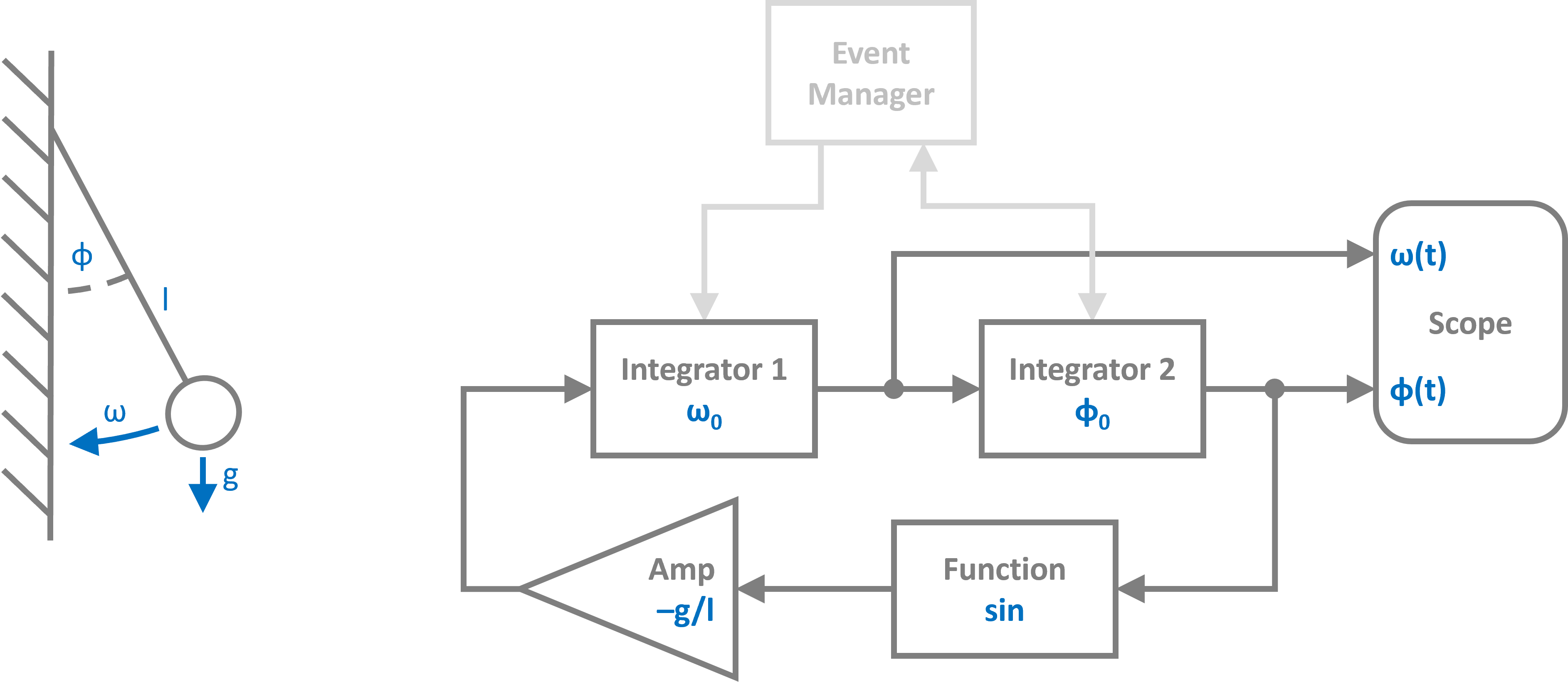
Block Diagram Construction

We construct the system from basic blocks:

# Blocks that define the system
In1 = Integrator(omega0)  # angular acceleration -> angular velocity
In2 = Integrator(phi0)    # angular velocity -> angle
Amp = Amplifier(-g/l)     # gravity term
Fnc = Function(np.sin)    # nonlinearity
Sco = Scope(labels=[r"$\omega$", r"$\phi$"])

blocks = [In1, In2, Amp, Fnc, Sco]

# Connections between the blocks
connections = [
    Connection(In1, In2, Sco[0]),
    Connection(In2, Fnc, Sco[1]),
    Connection(Fnc, Amp),
    Connection(Amp, In1)
]

Event Detection and Action

We define a ZeroCrossing event to detect when the pendulum hits the ground ($phi = 0$). The event function monitors the angle, and the action function reverses the angular velocity with an energy loss factor.

# Event function for zero crossing detection
def func_evt(t):
    *_, ph = In2()
    return ph

# Action function for state transformation
def func_act(t):
    *_, om = In1()
    *_, ph = In2()
    In1.engine.set(-om*b)  # reverse velocity with energy loss
    In2.engine.set(abs(ph))  # ensure angle stays positive

# Events (zero crossing)
E1 = ZeroCrossing(
    func_evt=func_evt,
    func_act=func_act,
    tolerance=1e-6
)

events = [E1]

The engine.set() method allows direct manipulation of block states during event actions. This is crucial for implementing the discontinuous velocity change at the bounce.

We initialize the simulation with the RKCK54 solver for accurate integration of the nonlinear dynamics:

# Simulation instance from the blocks and connections
Sim = Simulation(
    blocks,
    connections,
    events,
    dt=0.1,
    log=True,
    Solver=RKCK54,
    tolerance_lte_abs=1e-8,
    tolerance_lte_rel=1e-6
)

10:57:29 - INFO - LOGGING (log: True)
10:57:29 - INFO - BLOCKS (total: 5, dynamic: 2, static: 3, eventful: 0)
10:57:29 - INFO - GRAPH (nodes: 5, edges: 6, alg. depth: 3, loop depth: 0, runtime: 0.070ms)

Now let’s run the simulation:

Sim.run(duration=15)

10:57:29 - INFO - STARTING -> TRANSIENT (Duration: 15.00s)
10:57:29 - INFO - --------------------   1% | 0.0s<0.2s | 1358.8 it/s
10:57:29 - INFO - FINISHED -> TRANSIENT (total steps: 26, successful: 19, runtime: 25.15 ms)

---------------------------------------------------------------------------
NameError                                 Traceback (most recent call last)
Cell In[6], line 1
----> 1 Sim.run(duration=15)

File ~/checkouts/readthedocs.org/user_builds/pathsim/envs/v0.12.4/lib/python3.13/site-packages/pathsim/simulation.py:1754, in Simulation.run(self, duration, reset, adaptive)
   1751     break
   1753 #advance the simulation by one (effective) timestep '_dt'
-> 1754 success, error_norm, scale, *_ = self.timestep(
   1755     dt=_dt, 
   1756     adaptive=_adaptive
   1757     )
   1759 #perform adaptive rescale
   1760 if _adaptive:
   1761
   1762     #if no error estimate and rescale -> back to default timestep

File ~/checkouts/readthedocs.org/user_builds/pathsim/envs/v0.12.4/lib/python3.13/site-packages/pathsim/simulation.py:1646, in Simulation.timestep(self, dt, adaptive)
   1644 if adaptive and self.engine.is_adaptive:
   1645     if self.engine.is_explicit:
-> 1646         return self.timestep_adaptive_explicit(dt)
   1647     else:
   1648         return self.timestep_adaptive_implicit(dt)

File ~/checkouts/readthedocs.org/user_builds/pathsim/envs/v0.12.4/lib/python3.13/site-packages/pathsim/simulation.py:1489, in Simulation.timestep_adaptive_explicit(self, dt)
   1485 for event, close, ratio in self._detected_events(time_dt):
   1486
   1487     #close enough to event (ratio approx 1.0) -> resolve it
   1488     if close:
-> 1489         event.resolve(time_dt)
   1491         #after resolve, evaluate system equation again -> propagate event
   1492         self._update(time_dt)

File ~/checkouts/readthedocs.org/user_builds/pathsim/envs/v0.12.4/lib/python3.13/site-packages/pathsim/events/_event.py:209, in Event.resolve(self, t)
    207 #action function for event resolution
    208 if self.func_act is not None:
--> 209     self.func_act(t)

Cell In[4], line 10, in func_act(t)
      8 *_, om = In1()
      9 *_, ph = In2()
---> 10 In1.engine.set(-om*b)  # reverse velocity with energy loss
     11 In2.engine.set(abs(ph))

NameError: name 'b' is not defined

Results

Let’s plot the angular velocity and angle over time, marking the bounce events:

# Plot the results directly from the scope
fig, ax = Sco.plot(lw=2)

plt.show()

The plot shows:

• The angle oscillates between 0 and some maximum value that decreases over time

• The angular velocity reverses sign at each bounce (vertical dashed lines)

• Energy is progressively lost with each bounce, leading to smaller oscillations

Sensitivity Analysis

Since we wrapped the bounceback coefficient in a Value instance, we can extract sensitivities of the system response with respect to this parameter:

# Read the recordings from the scope
time, [om, ph] = Sco.read()

# Extract sensitivities
dom_db = Value.der(om, b)
dph_db = Value.der(ph, b)

# Plot sensitivities
fig, ax = plt.subplots(figsize=(8, 4), tight_layout=True, dpi=120)

ax.plot(time, dom_db, lw=2, c="tab:red", label=r"$\partial \omega / \partial b$")
ax.plot(time, dph_db, lw=2, c="tab:blue", label=r"$\partial \phi / \partial b$")

ax.set_xlabel("time [s]")
ax.legend()
ax.grid(True)

plt.show()

---------------------------------------------------------------------------
NameError                                 Traceback (most recent call last)
Cell In[8], line 5
      2 time, [om, ph] = Sco.read()
      4 # Extract sensitivities
----> 5 dom_db = Value.der(om, b)
      6 dph_db = Value.der(ph, b)
      8 # Plot sensitivities

NameError: name 'Value' is not defined

These sensitivities show how changes in the bounceback coefficient would affect the angular velocity and angle trajectories. This is particularly useful for:

• Understanding parameter influence on hybrid system behavior

• Optimization of system parameters

• Uncertainty quantification when the bounceback coefficient has measurement uncertainty

PathSim’s automatic differentiation framework propagates gradients through both continuous dynamics and discrete events, making sensitivity analysis of hybrid systems straightforward.