Diode Circuit

You can also find this example as a single file in the GitHub repository.This example demonstrates a more complex application of algebraic loop solving: a diode circuit with nonlinear characteristics. This showcases PathSim’s ability to handle nonlinear implicit equations that arise in real electronic circuits.

Circuit Description

The circuit consists of:

• A sinusoidal voltage source: \(V_s(t) = 5\sin(2\pi t)\) V

• A resistor: \(R = 1000\) Ω

• A diode with exponential I-V characteristic

Diode Model

The diode current follows the Shockley equation:

\[i_D = I_s \left(e^{V_D/V_T} - 1\right)\]

Where:

• \(I_s = 10^{-12}\) A (saturation current)

• \(V_T = 26\) mV (thermal voltage at room temperature)

• \(V_D\) is the diode voltage

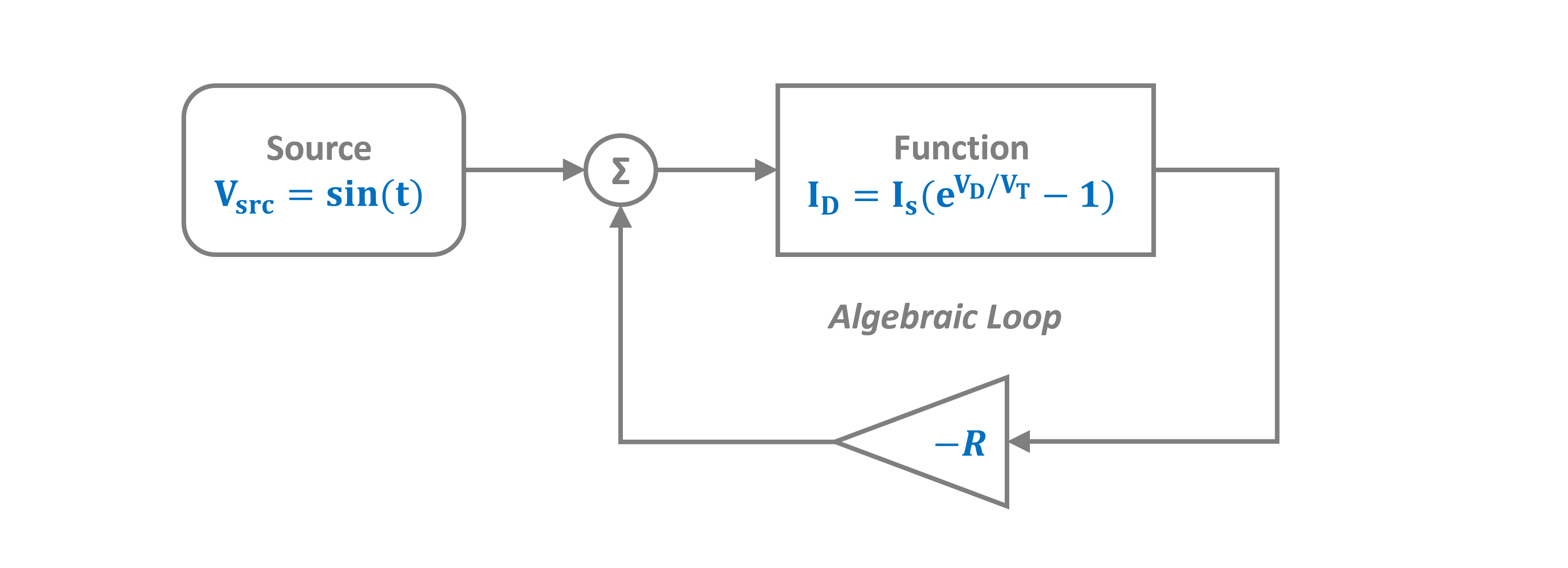
The Algebraic Loop

Applying Kirchhoff’s Voltage Law (KVL):

\[V_s = V_D + R \cdot i_D\]

Substituting the diode equation creates a nonlinear algebraic loop:

\[V_D = V_s - R \cdot I_s \left(e^{V_D/V_T} - 1\right)\]

PathSim solves this nonlinear equation automatically at each timestep using accelerated fixed-point iteration.

This example demonstrates a nonlinear algebraic loop. The Function block implements the diode characteristic, and PathSim solves the implicit circuit equations automatically.

import numpy as np
import matplotlib.pyplot as plt

# Apply PathSim docs matplotlib style
plt.style.use('../pathsim_docs.mplstyle')

from pathsim import Simulation, Connection
from pathsim.blocks import Source, Amplifier, Function, Adder, Scope
from pathsim.solvers import RKBS32

Circuit Parameters

# Circuit parameters
R = 1000.0          # Resistor (Ohms)
I_s = 1e-12         # Diode saturation current (A)
V_T = 0.026         # Thermal voltage at room temperature (V)

# Define diode current function: i = I_s * (exp(v_diode/(V_T)) - 1)
def diode_current(v_diode):
    """Diode current as function of diode voltage"""
    # Clip to prevent numerical overflow
    clipped = np.clip(v_diode/V_T, None, 23)
    return I_s * (np.exp(clipped) - 1)

# Define voltage source function
def voltage_source(t):
    """Sinusoidal voltage source"""
    return 5.0 * np.sin(2 * np.pi * t)

# Blocks that define the system
Src = Source(voltage_source)                    # Voltage source
DiodeFn = Function(diode_current)               # Diode i-v characteristic
ResAmp = Amplifier(-R)                          # -R (negative resistance)
Add = Adder()                                   # Adder for KVL
Sc1 = Scope(labels=["v_source", "v_diode"])
Sc2 = Scope(labels=["i_diode"])

blocks = [Src, DiodeFn, ResAmp, Add, Sc1, Sc2]

Connections

The connections implement Kirchhoff’s laws:

• The adder computes: \(V_{diode} = V_{source} + V_{resistor}\)

• The resistor voltage is: \(V_{resistor} = -R \cdot i_{diode}\)

• The diode current depends on: \(V_{diode}\) (creating the loop)

connections = [
    Connection(Src, Add[0], Sc1[0]),            # Source to adder and scope
    Connection(Add, DiodeFn, Sc1[1]),           # Diode voltage to function and scope
    Connection(DiodeFn, ResAmp, Sc2),           # Diode current to resistor and scope
    Connection(ResAmp, Add[1]),                 # Voltage drop back to adder (loop!)
]

Simulation

We use a tight convergence tolerance (tolerance_fpi=1e-12) to ensure accurate solution of the nonlinear algebraic equation.

# Simulation instance
Sim = Simulation(
    blocks,
    connections,
    dt=0.001,
    tolerance_fpi=1e-12
)

# Run the simulation for 2 seconds
Sim.run(duration=2.0)

12:11:45 - INFO - LOGGING (log: True)
12:11:45 - INFO - BLOCKS (total: 6, dynamic: 0, static: 6, eventful: 0)
12:11:45 - INFO - GRAPH (nodes: 6, edges: 7, alg. depth: 1, loop depth: 3, runtime: 0.096ms)
12:11:45 - INFO - STARTING -> TRANSIENT (Duration: 2.00s)
12:11:45 - INFO - --------------------   1% | 0.0s<0.9s | 2093.6 it/s
12:11:45 - ERROR - algebraic loop not converged (iters: 200, err: 1.787475614641897)
12:11:45 - INFO - FINISHED -> TRANSIENT (total steps: 57, successful: 57, runtime: 60.54 ms)

---------------------------------------------------------------------------
RuntimeError                              Traceback (most recent call last)
Cell In[5], line 10
      2 Sim = Simulation(
      3     blocks,
      4     connections,
      5     dt=0.001,
      6     tolerance_fpi=1e-12
      7 )
      9 # Run the simulation for 2 seconds
---> 10 Sim.run(duration=2.0)

File ~/checkouts/readthedocs.org/user_builds/pathsim/envs/v0.12.0/lib/python3.13/site-packages/pathsim/simulation.py:1771, in Simulation.run(self, duration, reset, adaptive)
   1768     break
   1770 #advance the simulation by one (effective) timestep '_dt'
-> 1771 success, error_norm, scale, *_ = self.timestep(
   1772     dt=_dt, 
   1773     adaptive=_adaptive
   1774     )
   1776 #perform adaptive rescale
   1777 if _adaptive:
   1778
   1779     #if no error estimate and rescale -> back to default timestep

File ~/checkouts/readthedocs.org/user_builds/pathsim/envs/v0.12.0/lib/python3.13/site-packages/pathsim/simulation.py:1668, in Simulation.timestep(self, dt, adaptive)
   1666 else:
   1667     if self.engine.is_explicit:
-> 1668         return self.timestep_fixed_explicit(dt)
   1669     else:
   1670         return self.timestep_fixed_implicit(dt)

File ~/checkouts/readthedocs.org/user_builds/pathsim/envs/v0.12.0/lib/python3.13/site-packages/pathsim/simulation.py:1310, in Simulation.timestep_fixed_explicit(self, dt)
   1307 time_dt = self.time + dt
   1309 #evaluate system equation before sampling and event check (+dt)
-> 1310 self._update(time_dt)
   1311 total_evals += 1
   1313 #handle events chronologically after timestep (+dt)

File ~/checkouts/readthedocs.org/user_builds/pathsim/envs/v0.12.0/lib/python3.13/site-packages/pathsim/simulation.py:935, in Simulation._update(self, t)
    933 #algebraic loops -> solve them
    934 if self.graph.has_loops:
--> 935     self._loops(t)

File ~/checkouts/readthedocs.org/user_builds/pathsim/envs/v0.12.0/lib/python3.13/site-packages/pathsim/simulation.py:1003, in Simulation._loops(self, t)
    999 _msg = "algebraic loop not converged (iters: {}, err: {})".format(
   1000     self.iterations_max, max_err
   1001     )
   1002 self.logger.error(_msg)
-> 1003 raise RuntimeError(_msg)

RuntimeError: algebraic loop not converged (iters: 200, err: 1.787475614641897)

Results: Voltage Waveforms

The plots show:

• v_source (blue): Input sinusoidal voltage

• v_diode (orange): Voltage across the diode

Notice how the diode voltage is:

• Clamped near ~0.7V during forward bias (positive half-cycle)

• Follows the source during reverse bias (negative half-cycle, diode is off)

This is the classic diode rectifier behavior!

Sim.plot()
plt.show()

Diode Current

Let’s examine the diode current to see the rectification more clearly.

# Get results
time, [i_diode] = Sc2.read()

fig, ax = plt.subplots(figsize=(8, 4))
ax.plot(time, i_diode * 1000, linewidth=2)  # Convert to mA
ax.set_xlabel('Time [s]')
ax.set_ylabel('Diode Current [mA]')
ax.set_title('Diode Current (Half-Wave Rectification)')
ax.grid(True, alpha=0.3)
ax.axhline(y=0, color='k', linestyle='--', linewidth=0.8)
plt.tight_layout()
plt.show()

Diode I-V Characteristic

We can also visualize the diode’s I-V characteristic by plotting current vs. voltage.

# Get diode voltage
_, [v_source, v_diode] = Sc1.read()

# Plot I-V characteristic
fig, ax = plt.subplots(figsize=(8, 4))

ax.axhline(y=0, color='grey', linestyle='--', linewidth=1.8)
ax.axvline(x=0, color='grey', linestyle='--', linewidth=1.8)

ax.plot(v_diode, i_diode * 1000, '.', markersize=3, alpha=0.5)

ax.set_xlabel('Diode Voltage [V]')
ax.set_ylabel('Diode Current [mA]')
ax.set_title('Diode I-V Characteristic (Dynamic Load Line)')
ax.grid(True, alpha=0.3)
plt.tight_layout()
plt.show()