Van der Pol
Here we cover a true classic from the worldof dynamical systems. The Van der Pol system!
You can also find this example as a single file in the GitHub repository.
It is described by the following 2nd order ODE
where the parameter \(\mu\) controles the stiffness of the system. Stiffness in dynamical systems typically arises when the (local) internal time constants (eigenvalues of the Jacobian) are on different scales, or when very steep gradients are encountered.
ODE solvers for stiff systems require large stability regions and therefore are usually implicit. PathSim has a huge range of implicit solvers (i.e. ESDIRK32, ESDIRK43, GEAR52A, …), that can be used to solve stiff systems, such as the Van der Pol system with very large \(\mu\), reliably. Lets see how this works.
PathSim supplies a specific block to define differential equations, the ODE block. To accept the Van der Pol system, we have to convert the 2nd order ODE into a system of 1st order ODEs:
As a block diagram it would look like this:
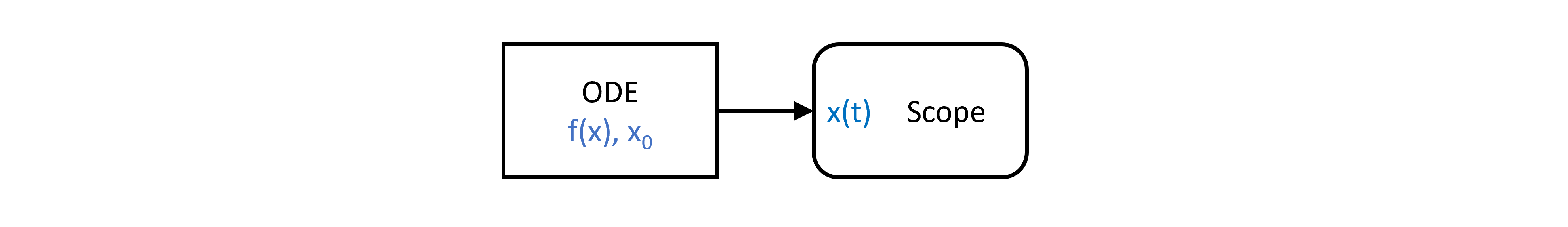
And translated to PathSim like this:
from pathsim import Simulation, Connection
from pathsim.blocks import Scope, ODE
from pathsim.solvers import GEAR52A # <- implicit solver for stiff systems

#initial condition
x0 = np.array([2, 0])

#van der Pol parameter
mu = 1000 # <- this is very stiff

def func(x, u, t):
    return np.array([x[1], mu*(1 - x[0]**2)*x[1] - x[0]])

#analytical jacobian (optional)
def jac(x, u, t):
    return np.array([[0, 1], [-mu*2*x[0]*x[1]-1, mu*(1 - x[0]**2)]])

#blocks that define the system
VDP = ODE(func, x0, jac) #jacobian improves convergence
Sco = Scope(labels=[r"$x_1(t)$"])

blocks = [VDP, Sco]

#the connect the blocks
connections = [
    Connection(VDP, Sco)
    ]

#initialize simulation
Sim = Simulation(
    blocks,
    connections,
    Solver=GEAR52A,
    tolerance_lte_abs=1e-5,
    tolerance_lte_rel=1e-3,
    tolerance_fpi=1e-8
    )
Here we define the paramter \(\mu = 1000\) (btw. \(\mu = 10000\) also works), which means severe stiffness! This is pretty much a torture test for stiff ODE solvers.
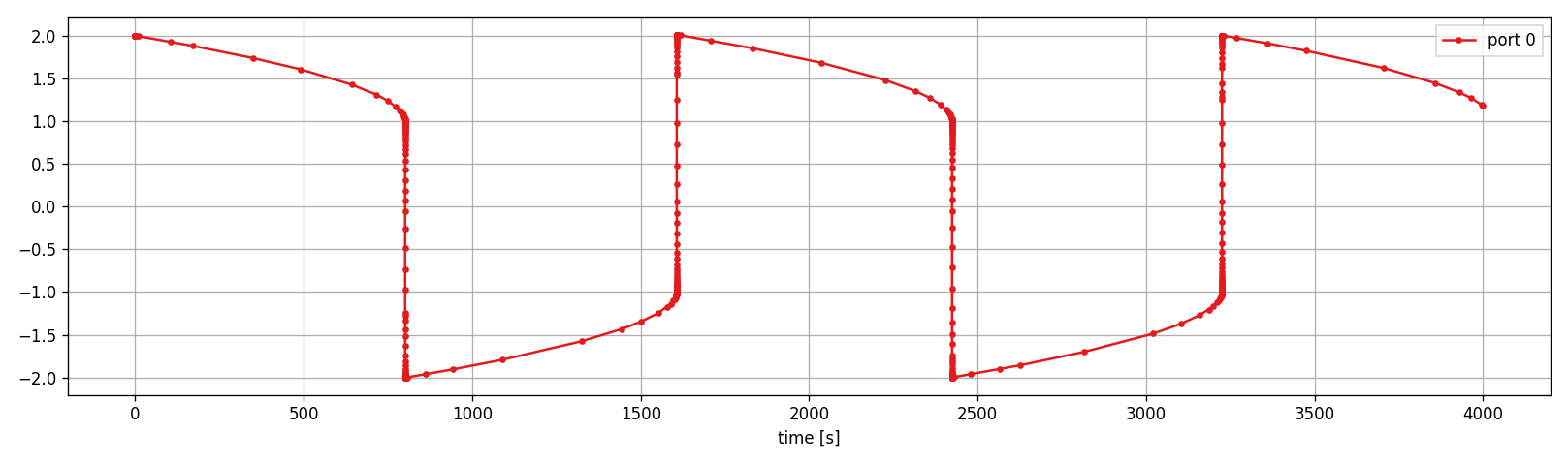
Lets run the simulation and look at the results:
#run it
Sim.run(4*mu)

#plotting
Sco.plot(".-")
Van der Pol - as a Subsystem
Of course we dont have to use the ODE block to implement the Van der Pol system. We can also use other native PathSim blocks to achieve the same result!
This is the right moment to talk about PathSim hierarchical modeling capability. The Subsystem class enables the encapsulation of blocks and connections such that they can be treated as a single block from the outside.
Lets use a Subsystem with distinct internal blocks and connections to emulate the ODE block from above. In the block diagram paradigm this might look like this:
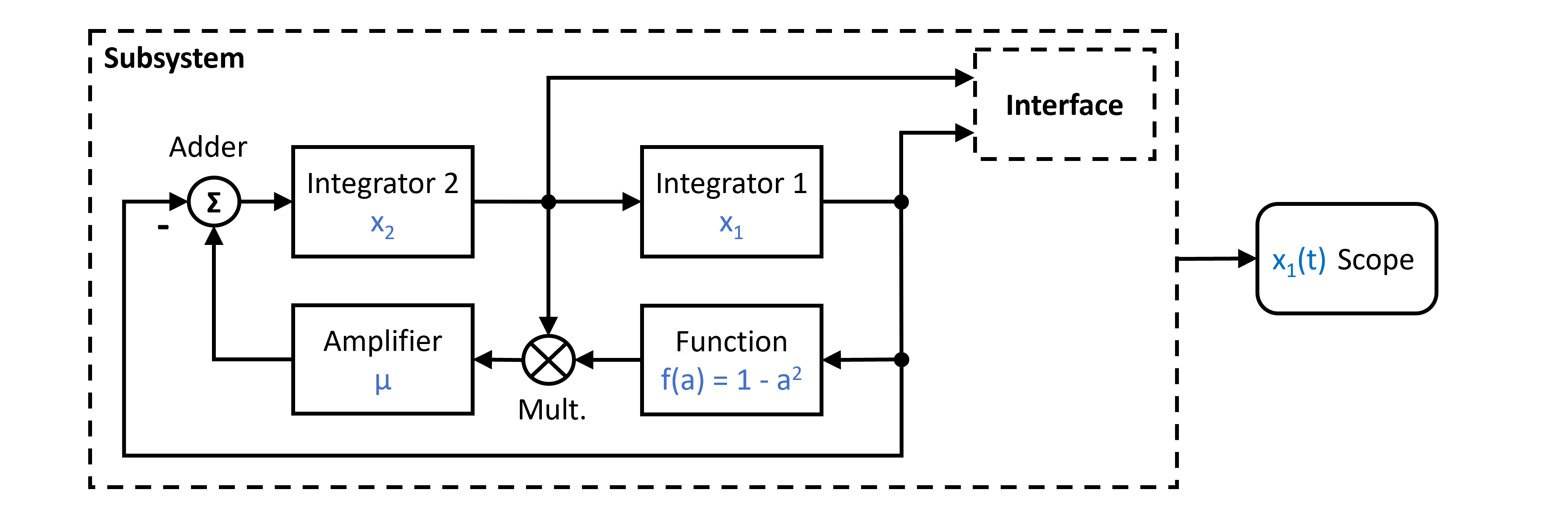
To translate it to PathSim, lets first build the Van der Pol block as a Subsystem (visit GitHub for this example to run it yourself):
from pathsim import Simulation, Connection, Interface, Subsystem
from pathsim.blocks import Integrator, Scope, Adder, Multiplier, Amplifier, Function
from pathsim.solvers import GEAR52A # <- implicit solver for stiff systems

#initial condition
x1_0 = 2
x2_0 = 0

#van der Pol parameter
mu = 1000

#subsystem to emulate ODE block
If = Interface()
I1 = Integrator(x1_0)
I2 = Integrator(x2_0)
Fn = Function(lambda a: 1 - a**2)
Pr = Multiplier()
Ad = Adder("-+")
Am = Amplifier(mu)

sub_blocks = [If, I1, I2, Fn, Pr, Ad, Am]
sub_connections = [
    Connection(I2, I1, Pr[0], If[1]),
    Connection(I1, Fn, Ad[0], If[0]),
    Connection(Fn, Pr[1]),
    Connection(Pr, Am),
    Connection(Am, Ad[1]),
    Connection(Ad, I2)
    ]

#the subsystem acts just like a normal block
VDP = Subsystem(sub_blocks, sub_connections)
Subsystems in PathSim hold their own internal blocks and connections. The communication to the outside is realized by a special Interface block, that the internal blocks are connected to. The inputs of this block are passed to the outputs of the Subsystem and the inputs of the Subsystem are passed to the outputs of the Interface.
Now, VDP behaves just like the ODE block from above. Lets continue with the top level system:
#blocks of the main system
blocks = [VDP, Sco]

#the connections between the blocks in the main system
connections = [
    Connection(VDP, Sco)
    ]

#initialize simulation with the blocks, connections, timestep and logging enabled
Sim = Simulation(
    blocks,
    connections,
    Solver=GEAR52A,
    tolerance_lte_abs=1e-5,
    tolerance_lte_rel=1e-3,
    tolerance_fpi=1e-8
    )
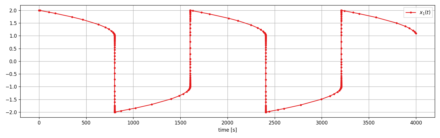
Run the simulation and see what happens:
#run it
Sim.run(4*mu)

#plotting
Sco.plot(".-")