Kalman Filter

This example demonstrates the Kalman filter in PathSim for optimal state estimation of a linear dynamical system from noisy measurements. The filter recursively estimates the state of a moving object by combining predictions from a system model with noisy sensor measurements.

You can also find this example as a single file in the GitHub repository.

Import and Setup

First let’s import the required classes and blocks:

import numpy as np
import matplotlib.pyplot as plt

# Apply PathSim docs matplotlib style
plt.style.use('../pathsim_docs.mplstyle')

from pathsim import Simulation, Connection
from pathsim.blocks import (
    Constant,
    Integrator,
    Adder,
    WhiteNoise,
    KalmanFilter,
    Scope
)

System Parameters

We simulate a simple object moving with constant velocity. The true system has a velocity of 2 m/s, but we can only measure its position with noisy sensors. The Kalman filter will estimate both position and velocity from the noisy position measurements.

# Simulation parameters
dt = 0.01  # timestep

# True system: object moving with constant velocity
v_true = 2.0   # m/s
x0_true = 0.0  # initial position

# Measurement noise characteristics
measurement_std = 0.6  # standard deviation of position sensor noise

Kalman Filter Configuration

The Kalman filter requires several matrices:

• F: State transition matrix (how the state evolves)

• H: Measurement matrix (what we can observe)

• Q: Process noise covariance (model uncertainty)

• R: Measurement noise covariance (sensor uncertainty)

• x0: Initial state estimate

• P0: Initial error covariance

# Kalman filter parameters
F = np.array([[1, dt], [0, 1]])        # state transition (constant velocity model)
H = np.array([[1, 0]])                 # measurement matrix (measure position only)

# Process noise covariance - models uncertainty in constant velocity assumption
# Derived from continuous-time noise with intensity q = 0.1
q = 0.1  # process noise intensity (m/s^2)^2
Q = np.array([
    [dt**3/3, dt**2/2],
    [dt**2/2, dt]
]) * q

R = np.array([[measurement_std**2]])   # measurement noise covariance
x0_kf = np.array([0, 0])               # initial estimate [position, velocity]
P0_kf = np.diag([1.0, 1.0])            # initial covariance

System Definition

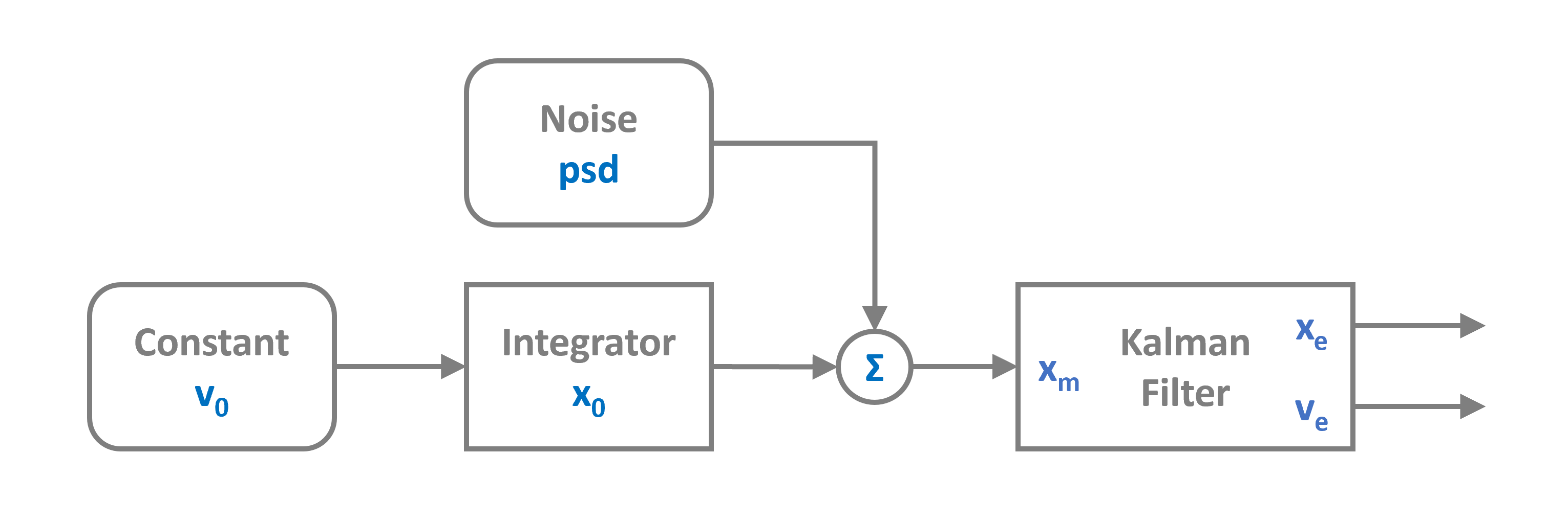
Now we construct the complete system including:

• The true system (constant velocity integrator)

• Noisy measurement sensor

• Kalman filter for state estimation

# True system
vel = Constant(v_true)
pos = Integrator(x0_true)

# Noisy measurement (spectral_density must be scaled by dt for discrete-time white noise)
noise = WhiteNoise(spectral_density=measurement_std**2 * dt)
measured_pos = Adder()

# Kalman filter
kf = KalmanFilter(F, H, Q, R, x0=x0_kf, P0=P0_kf)

# Scopes for recording
sc_true = Scope(labels=["true position", "true velocity"])
sc_meas = Scope(labels=["measured position"])
sc_est = Scope(labels=["estimated position", "estimated velocity"])

blocks = [vel, pos, noise, measured_pos, kf, sc_true, sc_meas, sc_est]

The WhiteNoise block adds Gaussian noise to the true position measurement. The KalmanFilter processes these noisy measurements to estimate both position and velocity.

# Connections
connections = [
    Connection(vel, pos, sc_true[1]),
    Connection(pos, measured_pos[0], sc_true[0]),
    Connection(noise, measured_pos[1]),
    Connection(measured_pos, kf, sc_meas),
    Connection(kf[0], sc_est[0]),
    Connection(kf[1], sc_est[1])
]

Simulation Setup and Execution

# Initialize simulation
Sim = Simulation(
    blocks,
    connections,
    dt=dt,
)

# Run the simulation for 20 seconds
Sim.run(duration=20)

11:40:25 - INFO - LOGGING (log: True)
11:40:25 - INFO - BLOCKS (total: 8, dynamic: 1, static: 7, eventful: 0)
11:40:25 - INFO - GRAPH (nodes: 8, edges: 9, alg. depth: 2, loop depth: 0, runtime: 0.042ms)
11:40:25 - INFO - STARTING -> TRANSIENT (Duration: 20.00s)
11:40:25 - INFO - --------------------   1% | 0.0s<0.2s | 10467.4 it/s
11:40:25 - INFO - ####----------------  20% | 0.0s<0.1s | 11160.1 it/s
11:40:26 - INFO - ########------------  40% | 0.1s<0.1s | 11027.6 it/s
11:40:26 - INFO - ############--------  60% | 0.1s<0.1s | 11414.2 it/s
11:40:26 - INFO - ################----  80% | 0.1s<0.0s | 11601.0 it/s
11:40:26 - INFO - #################### 100% | 0.2s<--:-- | 11416.4 it/s
11:40:26 - INFO - FINISHED -> TRANSIENT (total steps: 2000, successful: 2000, runtime: 183.78 ms)

{'total_steps': 2000,
 'successful_steps': 2000,
 'runtime_ms': 183.7788279999586}

Results: State Tracking

Let’s visualize how well the Kalman filter tracks the true position and velocity:

# Read data from scopes
t_true, [pos_true, vel_true] = sc_true.read()
t_meas, [pos_meas] = sc_meas.read()
t_est, [pos_est, vel_est] = sc_est.read()

# Create comparison plots
fig, (ax1, ax2) = plt.subplots(2, 1, figsize=(8, 6), tight_layout=True, dpi=200)

# Position comparison
ax1.set_title('Kalman Filter: Position and Velocity Estimation')
ax1.plot(t_meas, pos_meas, ".", label='Noisy Measurement')
ax1.plot(t_true, pos_true, "-", label='True Position')
ax1.plot(t_est, pos_est, "--", label='Kalman Estimate')
ax1.set_ylabel('Position [m]')
ax1.legend()

# Velocity comparison
ax2.plot(t_true, vel_true, "-", label='True Velocity')
ax2.plot(t_est, vel_est, "--", label='Kalman Estimate')
ax2.set_ylabel('Velocity [m/s]')
ax2.set_xlabel('Time [s]')
ax2.legend()

plt.show()

Estimation Error Analysis

Now let’s quantify the estimation accuracy by computing and plotting the absolute errors:

# Calculate estimation errors
pos_error = np.abs(pos_est - pos_true)
vel_error = np.abs(vel_est - vel_true)

# Estimation error over time
fig2, (ax3, ax4) = plt.subplots(2, 1, figsize=(8, 6), tight_layout=True, dpi=200)

ax3.plot(t_est, pos_error)
ax3.set_ylabel('Position Error [m]')
ax3.set_title('Kalman Filter Estimation Error')

ax4.plot(t_est, vel_error)
ax4.set_ylabel('Velocity Error [m/s]')
ax4.set_xlabel('Time [s]')

plt.show()