Diode Circuit

Simulation of a diode circuit demonstrating nonlinear algebraic loop solving.

You can also find this example as a single file in the GitHub repository.

Circuit Description

The circuit consists of:

• A sinusoidal voltage source: \(V_s(t) = 5\sin(2\pi t)\) V

• A resistor: \(R = 1000\) Ω

• A diode with exponential I-V characteristic

Diode Model

The diode current follows the Shockley equation:

\[i_D = I_s \left(e^{V_D/V_T} - 1\right)\]

Where:

• \(I_s = 10^{-12}\) A (saturation current)

• \(V_T = 26\) mV (thermal voltage at room temperature)

• \(V_D\) is the diode voltage

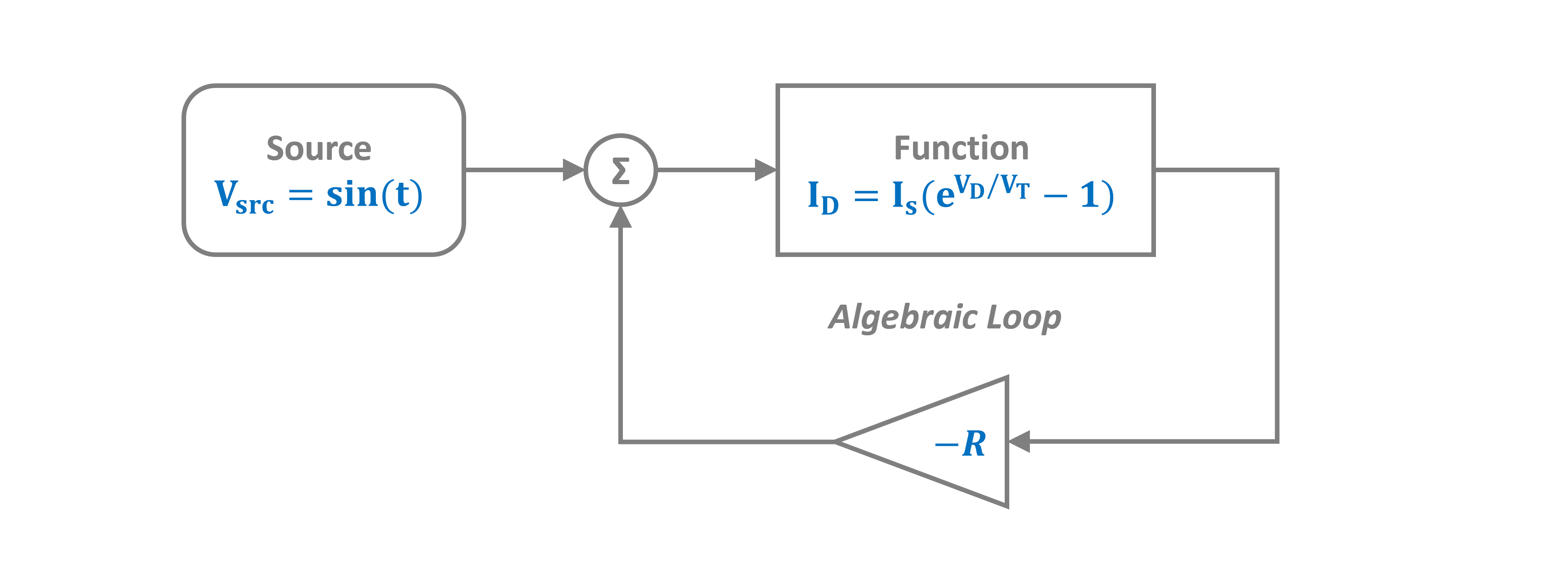
The Algebraic Loop

Applying Kirchhoff’s Voltage Law (KVL):

\[V_s = V_D + R \cdot i_D\]

Substituting the diode equation creates a nonlinear algebraic loop:

\[V_D = V_s - R \cdot I_s \left(e^{V_D/V_T} - 1\right)\]

PathSim solves this nonlinear equation automatically at each timestep using accelerated fixed-point iteration.

This example demonstrates a nonlinear algebraic loop. The Function block implements the diode characteristic, and PathSim solves the implicit circuit equations automatically.

import numpy as np
import matplotlib.pyplot as plt

# Apply PathSim docs matplotlib style
plt.style.use('../pathsim_docs.mplstyle')

from pathsim import Simulation, Connection
from pathsim.blocks import Source, Amplifier, Function, Adder, Scope

Circuit Parameters

# Circuit parameters
R = 1000.0          # Resistor (Ohms)
I_s = 1e-12         # Diode saturation current (A)
V_T = 0.026         # Thermal voltage at room temperature (V)

# Define diode current function: i = I_s * (exp(v_diode/(V_T)) - 1)
def diode_current(v_diode):
    """Diode current as function of diode voltage"""
    # Clip to prevent numerical overflow
    clipped = np.clip(v_diode/V_T, None, 23)
    return I_s * (np.exp(clipped) - 1)

# Define voltage source function
def voltage_source(t):
    """Sinusoidal voltage source"""
    return 5.0 * np.sin(2 * np.pi * t)

# Blocks that define the system
Src = Source(voltage_source)                    # Voltage source
DiodeFn = Function(diode_current)               # Diode i-v characteristic
ResAmp = Amplifier(-R)                          # -R (negative resistance)
Add = Adder()                                   # Adder for KVL
Sc1 = Scope(labels=["v_source", "v_diode"])
Sc2 = Scope(labels=["i_diode"])

blocks = [Src, DiodeFn, ResAmp, Add, Sc1, Sc2]

Connections

The connections implement Kirchhoff’s laws:

• The adder computes: \(V_{diode} = V_{source} + V_{resistor}\)

• The resistor voltage is: \(V_{resistor} = -R \cdot i_{diode}\)

• The diode current depends on: \(V_{diode}\) (creating the loop)

connections = [
    Connection(Src, Add[0], Sc1[0]),            # Source to adder and scope
    Connection(Add, DiodeFn, Sc1[1]),           # Diode voltage to function and scope
    Connection(DiodeFn, ResAmp, Sc2),           # Diode current to resistor and scope
    Connection(ResAmp, Add[1]),                 # Voltage drop back to adder (loop!)
]

Simulation

We use a tight convergence tolerance (tolerance_fpi=1e-12) to ensure accurate solution of the nonlinear algebraic equation.

# Simulation instance
Sim = Simulation(
    blocks,
    connections,
    dt=0.01,
    tolerance_fpi=1e-12
)

# Run the simulation for 2 seconds
Sim.run(duration=2.0)

08:30:47 - INFO - LOGGING (log: True)
08:30:47 - INFO - BLOCKS (total: 6, dynamic: 0, static: 6, eventful: 0)
08:30:47 - INFO - GRAPH (nodes: 6, edges: 7, alg. depth: 1, loop depth: 3, runtime: 0.085ms)
08:30:47 - INFO - STARTING -> TRANSIENT (Duration: 2.00s)
08:30:47 - INFO - --------------------   1% | 0.0s<0.2s | 873.7 it/s
08:30:47 - INFO - ####----------------  20% | 0.0s<0.1s | 1261.0 it/s
08:30:47 - INFO - ########------------  40% | 0.0s<0.0s | 27806.9 it/s
08:30:47 - INFO - ############--------  60% | 0.1s<0.1s | 1217.4 it/s
08:30:47 - INFO - ################----  80% | 0.1s<0.0s | 28989.0 it/s
08:30:47 - INFO - #################### 100% | 0.1s<--:-- | 24181.2 it/s
08:30:47 - INFO - FINISHED -> TRANSIENT (total steps: 200, successful: 200, runtime: 93.20 ms)

{'total_steps': 200, 'successful_steps': 200, 'runtime_ms': 93.1966589998865}

Results: Voltage Waveforms

The plots show:

• v_source (blue): Input sinusoidal voltage

• v_diode (orange): Voltage across the diode

Notice how the diode voltage is:

• Clamped near ~0.7V during forward bias (positive half-cycle)

• Follows the source during reverse bias (negative half-cycle, diode is off)

This is the classic diode rectifier behavior!

Sim.plot()
plt.show()

Diode Current

Let’s examine the diode current to see the rectification more clearly.

# Get results
time, [i_diode] = Sc2.read()

fig, ax = plt.subplots(figsize=(8, 4))
ax.plot(time, i_diode * 1000, linewidth=2)  # Convert to mA
ax.set_xlabel('Time [s]')
ax.set_ylabel('Diode Current [mA]')
ax.set_title('Diode Current (Half-Wave Rectification)')
ax.grid(True, alpha=0.3)
ax.axhline(y=0, color='k', linestyle='--', linewidth=0.8)
plt.tight_layout()
plt.show()

Diode I-V Characteristic

We can also visualize the diode’s I-V characteristic by plotting current vs. voltage.

# Get diode voltage
_, [v_source, v_diode] = Sc1.read()

# Plot I-V characteristic
fig, ax = plt.subplots(figsize=(8, 4))

ax.axhline(y=0, color='grey', linestyle='--', linewidth=1.8)
ax.axvline(x=0, color='grey', linestyle='--', linewidth=1.8)

ax.plot(v_diode, i_diode * 1000, '.', markersize=3, alpha=0.5)

ax.set_xlabel('Diode Voltage [V]')
ax.set_ylabel('Diode Current [mA]')
ax.set_title('Diode I-V Characteristic (Dynamic Load Line)')
ax.grid(True, alpha=0.3)
plt.tight_layout()
plt.show()