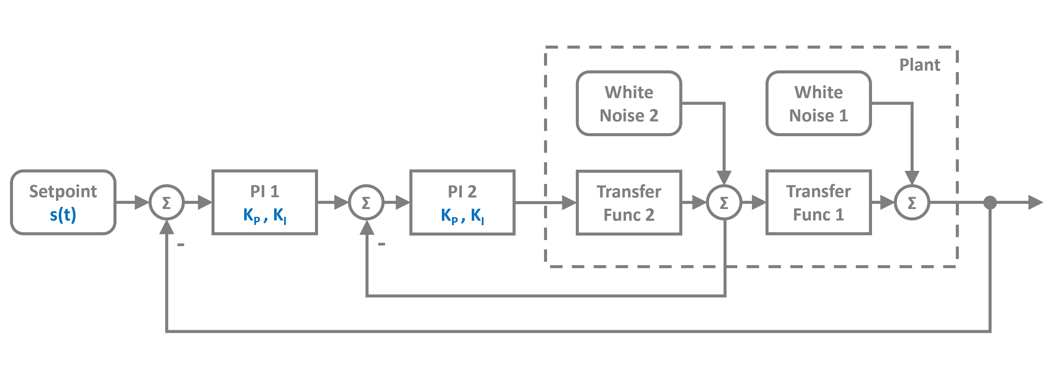
Cascade Controller

Demonstration of a two-loop cascade PID control system with inner and outer loops.

You can also find this example as a single file in the GitHub repository.

System Architecture

The cascade controller consists of:

• An outer loop (primary controller) that regulates the main process variable

• An inner loop (secondary controller) that controls an intermediate variable

• A plant modeled as a subsystem with two cascaded transfer functions and noise disturbances

The inner loop responds faster to disturbances, improving the overall system response.

First let’s import the Simulation, Connection, Subsystem, and Interface classes along with the required blocks:

import numpy as np
import matplotlib.pyplot as plt

# Apply PathSim docs matplotlib style
plt.style.use('../pathsim_docs.mplstyle')

from pathsim import Simulation, Connection, Subsystem, Interface
from pathsim.blocks import Source, TransferFunctionZPG, Adder, Scope, PID, WhiteNoise
from pathsim.solvers import RKCK54

Plant Definition

We define the plant as a Subsystem containing two cascaded transfer functions with noise disturbances. The plant uses TransferFunctionZPG blocks (zero-pole-gain representation) and WhiteNoise blocks for disturbances.

# Define the plant as a subsystem
in1 = Interface()

p1 = TransferFunctionZPG(Zeros=[], Poles=[-1, -1, -1], Gain=10)
p2 = TransferFunctionZPG(Zeros=[], Poles=[-2], Gain=3)

a1 = Adder()
a2 = Adder()

d1 = WhiteNoise(spectral_density=5e-7)
d2 = WhiteNoise(spectral_density=5e-7)

plant = Subsystem(
    blocks=[p1, p2, a1, a2, d1, d2, in1],
    connections=[
        Connection(in1, p2),
        Connection(p2, a2[0]),
        Connection(d2, a2[1]),
        Connection(a2, p1, in1[1]),
        Connection(p1, a1[0]),
        Connection(d1, a1[1]),
        Connection(a1, in1[0])
    ]
)

Control Loops

We set up two PID controllers:

• c1: Outer loop PID controller (primary)

• c2: Inner loop PID controller (secondary)

The inner controller is typically tuned to be faster than the outer controller. The setpoint changes at different time intervals to demonstrate the tracking performance.

# Source function with changing setpoints
def f_s(t):
    if t > 60:
        return 0.5
    elif t > 20:
        return 1
    else:
        return 0

stp = Source(f_s)

# PID controllers
c1 = PID(Kp=0.015, Ki=0.015/0.716, Kd=0.0, f_max=10.0)  # Outer loop
c2 = PID(Kp=0.244, Ki=0.244/0.134, Kd=0.0, f_max=10.0)  # Inner loop

# Error calculation blocks
e1 = Adder("+-")
e2 = Adder("+-")

# Scopes for monitoring
sc0 = Scope(labels=["setpoint", "plant 1", "plant 2"])
sc1 = Scope(labels=["err 1", "pid 1"])
sc2 = Scope(labels=["err 2", "pid 2"])

We initialize the simulation with all blocks and connections. We use the RKCK54 solver (Runge-Kutta-Cash-Karp 5(4) method) with adaptive time-stepping for accurate integration of the transfer function dynamics.

Sim = Simulation(
    blocks=[stp, plant, c1, c2, e1, e2, sc0, sc1, sc2],
    connections=[
        Connection(stp, e1[0], sc0[0]),
        Connection(plant[0], e1[1], sc0[1]),
        Connection(e1, c1, sc1[0]),
        Connection(c1, e2[0], sc1[1]),
        Connection(plant[1], e2[1], sc0[2]),
        Connection(e2, c2, sc2[0]),
        Connection(c2, plant, sc2[1])
    ],
    Solver=RKCK54,
    tolerance_lte_rel=1e-4,
    tolerance_lte_abs=1e-6
)

13:28:43 - INFO - LOGGING (log: True)
13:28:43 - INFO - BLOCKS (total: 9, dynamic: 3, static: 6, eventful: 0)
13:28:43 - INFO - GRAPH (nodes: 9, edges: 14, alg. depth: 5, loop depth: 0, runtime: 0.079ms)

Now let’s run the simulation for 100 seconds:

# Run the simulation
Sim.run(100)

13:28:43 - INFO - STARTING -> TRANSIENT (Duration: 100.00s)
13:28:43 - INFO - --------------------   1% | 0.0s<0.8s | 1431.9 it/s
13:28:43 - INFO - ####----------------  20% | 0.3s<01:51:41 | 1480.5 it/s
13:28:44 - INFO - ########------------  40% | 0.5s<0.6s | 1467.2 it/s
13:28:44 - INFO - ############--------  60% | 0.7s<27:46 | 1493.7 it/s
13:28:44 - INFO - ################----  80% | 0.9s<0.2s | 1472.9 it/s
13:28:44 - INFO - #################### 100% | 1.1s<--:-- | 1450.3 it/s
13:28:44 - INFO - FINISHED -> TRANSIENT (total steps: 1681, successful: 1233, runtime: 1146.95 ms)

{'total_steps': 1681,
 'successful_steps': 1233,
 'runtime_ms': 1146.9528169982368}

The Simulation class has a convenient plot method that plots all Scope blocks in the simulation:

# Plot all scopes
Sim.plot()
plt.show()