Nested Subsystems
You can also find this example as a single file in the GitHub repository.This example demonstrates PathSim’s hierarchical modeling capabilities using nested subsystems. We’ll build a complex Van der Pol oscillator by composing simpler subsystems, showing how to organize large models in a modular way.
Why Use Subsystems?
Subsystems allow you to:
Organize complex systems into logical modules
Reuse components across different models
Abstract implementation details
Scale to large systems with many components
Debug and test individual modules separately
The Van der Pol Oscillator Revisited
The stiff Van der Pol oscillator is described by:
With \(\mu = 1000\) (very stiff!)
Hierarchical Structure
This example demonstrates hierarchical modeling using Subsystem and Interface blocks for modular system design.
[1]:
import numpy as np
import matplotlib.pyplot as plt

# Apply PathSim docs matplotlib style for consistent, theme-friendly figures
plt.style.use('../pathsim_docs.mplstyle')

from pathsim import Simulation, Connection, Interface, Subsystem
from pathsim.blocks import Integrator, Scope, Function, Multiplier, Adder, Amplifier, Constant, Pow
from pathsim.solvers import ESDIRK43
System Parameters
[2]:
# Initial conditions
x1_0 = 2.0
x2_0 = 0.0

# Van der Pol parameter (high stiffness!)
mu = 1000

# Simulation timestep
dt = 0.01
Level 1: ODE Function Subsystem
First, we create a subsystem that computes \(f(x_1, x_2) = \mu(1 - x_1^2)x_2 - x_1\)
This subsystem:
Takes two inputs: \(x_1\) and \(x_2\)
Returns one output: the computed derivative
Is self-contained and reusable
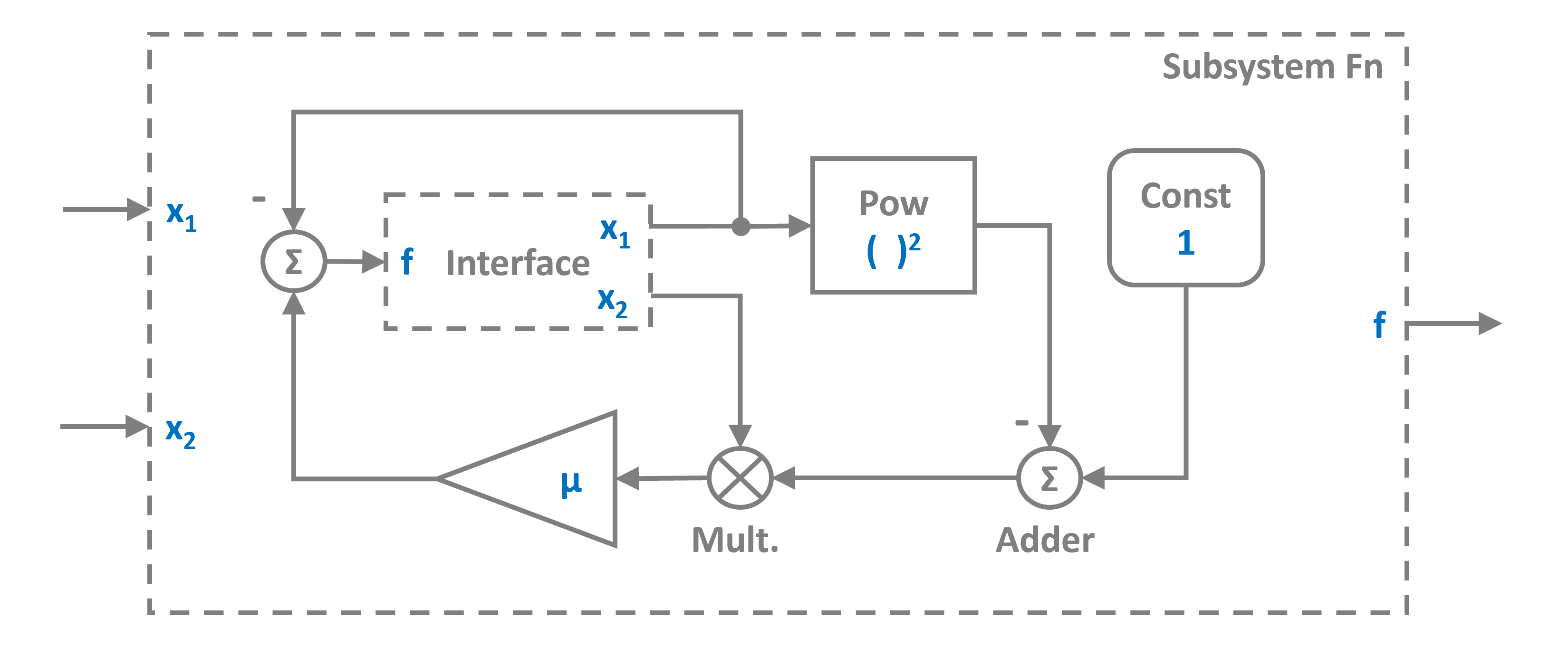
The Interface block defines the subsystem’s inputs and outputs and this is how it looks like in pathsim:
[3]:
# Interface for the ODE function subsystem
# Input 0: x1
# Input 1: x2
# Output: μ(1 - x1²)x2 - x1

In = Interface()
M1 = Multiplier()    # For x2 * (1 - x1²)
C1 = Constant(1)     # The constant 1
A1 = Amplifier(mu)   # Multiply by μ
P1 = Adder("+-")     # Sum: μ(1 - x1²)x2 - x1
P2 = Adder("+-")     # Compute: 1 - x1²
S1 = Pow(2)          # Square x1

fn_blocks = [In, M1, C1, A1, P1, P2, S1]

fn_connections = [
    Connection(In[0], S1),         # x1 → x1²
    Connection(In[1], M1[0]),      # x2 → multiplier
    Connection(S1, P2[1]),         # x1² to adder (-)
    Connection(C1, P2[0]),         # 1 to adder
    Connection(P2, M1[1]),         # (1 - x1²) to multiplier
    Connection(M1, A1),            # x2(1 - x1²) → multiply by μ
    Connection(A1, P1[0]),         # μ(...) to final adder
    Connection(In[0], P1[1]),      # x1 to final adder (-)
    Connection(P1, In)             # Result to output
]

# Create the ODE function subsystem
Fn = Subsystem(fn_blocks, fn_connections)
Level 2: Van der Pol Subsystem
Now we create a subsystem that contains:
Two integrators (for \(x_1\) and \(x_2\))
The ODE function subsystem we just created
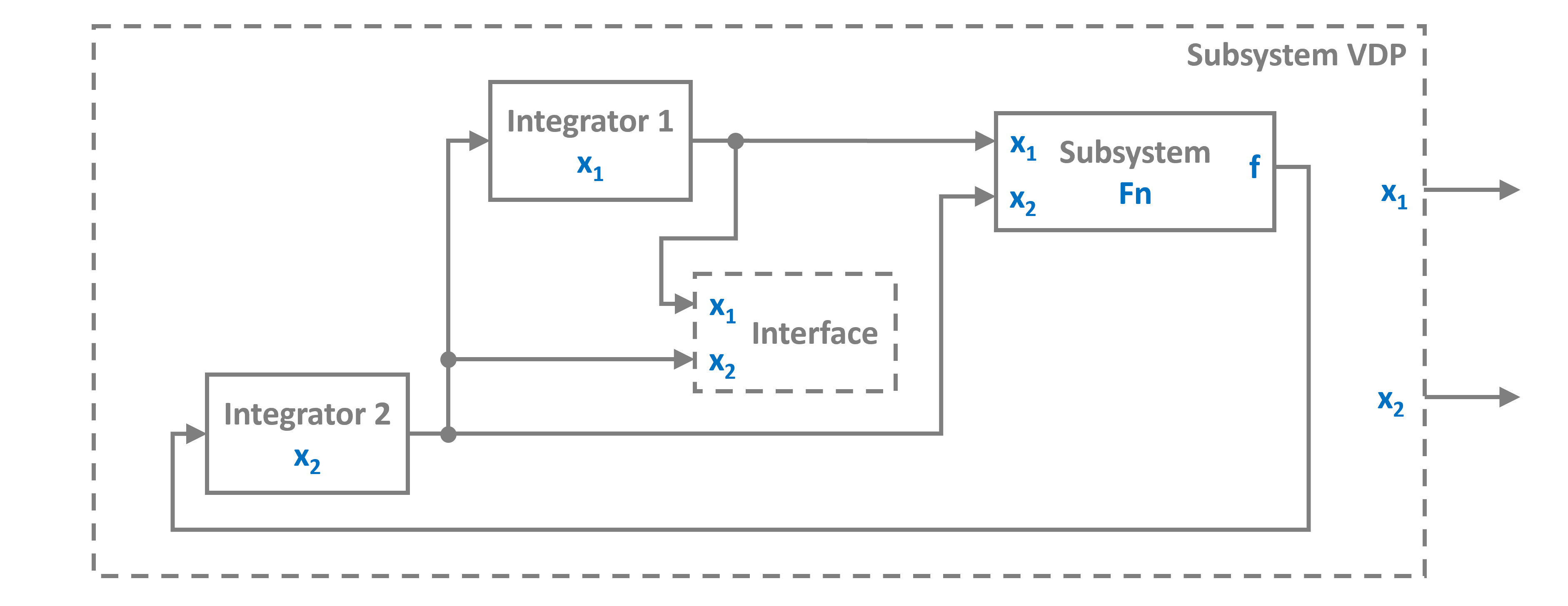
This implements the complete Van der Pol ODE system:
[4]:
# Interface for VDP subsystem (no inputs, two outputs)
If = Interface()
I1 = Integrator(x1_0)  # Integrator for x1
I2 = Integrator(x2_0)  # Integrator for x2

vdp_blocks = [If, I1, I2, Fn]

vdp_connections = [
    Connection(I2, I1, Fn[1], If[1]),  # x2 → I1, Fn, and output
    Connection(I1, Fn, If),            # x1 → Fn and output[0]
    Connection(Fn, I2)                 # dx2/dt → I2
]

# Create the Van der Pol subsystem
VDP = Subsystem(vdp_blocks, vdp_connections)
Level 3: Top-Level System
Finally, we create the top-level system that contains:
The VDP subsystem
A Scope for visualization
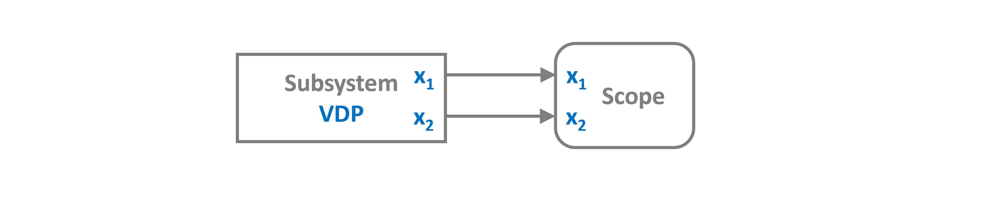
At this level, the VDP subsystem looks like a simple block with two outputs, hiding all its internal complexity
[5]:
# Top-level system
Sco = Scope(labels=[r"$x_1(t)$", r"$x_2(t)$"])

blocks = [VDP, Sco]

connections = [
    Connection(VDP, Sco),       # x1 to scope
    # Connection(VDP[1], Sco[1])  # x2 to scope
]
Simulation Setup
We use a stiff solver (ESDIRK43) because :math:`mu = 1000makes this a very stiff system.
[6]:
# Initialize simulation
Sim = Simulation(
    blocks,
    connections,
    dt=dt,
    log=True,
    Solver=ESDIRK43,
    tolerance_lte_abs=1e-6,
    tolerance_lte_rel=1e-4,
    tolerance_fpi=1e-7
)

# Run simulation (note: 2*mu for long-term dynamics)
Sim.run(2*mu)
17:30:40 - INFO - LOGGING (log: True)
17:30:40 - INFO - BLOCKS (total: 2, dynamic: 1, static: 1, eventful: 0)
17:30:40 - INFO - GRAPH (nodes: 2, edges: 1, alg. depth: 1, loop depth: 0, runtime: 0.013ms)
17:30:40 - INFO - STARTING -> TRANSIENT (Duration: 2000.00s)
17:30:40 - INFO - --------------------   1% | 0.3s<5.4s | 57.9 it/s
17:30:41 - INFO - #####---------------  28% | 0.5s<0.7s | 28.8 it/s
17:30:41 - INFO - ########------------  40% | 0.9s<7.1s | 47.3 it/s
17:30:42 - INFO - ########------------  41% | 2.0s<5.5s | 86.4 it/s
17:30:42 - INFO - #############-------  67% | 2.2s<0.3s | 39.8 it/s
17:30:43 - INFO - ################----  80% | 2.7s<2.0s | 41.6 it/s
17:30:44 - INFO - ################----  81% | 3.8s<2.5s | 90.5 it/s
17:30:44 - INFO - #################### 100% | 4.0s<--:-- | 45.8 it/s
17:30:44 - INFO - FINISHED -> TRANSIENT (total steps: 375, successful: 261, runtime: 3977.21 ms)
[6]:
{'total_steps': 375, 'successful_steps': 261, 'runtime_ms': 3977.205066999886}
Results: Time Series
The Van der Pol oscillator with \(\mu = 1000\) exhibits relaxation oscillations - fast transitions between slow phases. This requires a stiff solver to handle efficiently.
[7]:
Sco.plot(".-", lw=1.5)
plt.show()

Subsystem Benefits Demonstrated
This example shows several advantages of subsystems:
Modularity: The ODE function is completely separate from the integration
Reusability: The
Fnsubsystem could be used in other modelsClarity: The top level is clean - just VDP and Scope
Debugging: Each subsystem can be tested independently
Abstraction: Inner complexity is hidden from higher levels
Comparison with ODE Block
Compare this hierarchical approach with using a single ODE block:
# Alternative: Using ODE block (simpler but less modular)
def vdp_ode(x, u, t):
    return np.array([x[1], mu*(1 - x[0]**2)*x[1] - x[0]])

VDP = ODE(vdp_ode, np.array([x1_0, x2_0]))
Both approaches work! Use subsystems when:
You need modularity and reusability
The system is complex with many components
You want to visualize internal signals
You’re building block diagram models