Linear Feedback System

Here’s a simple example of a linear feedback system, simulated with PathSim.

You can also find this example as a single file in the GitHub repository.

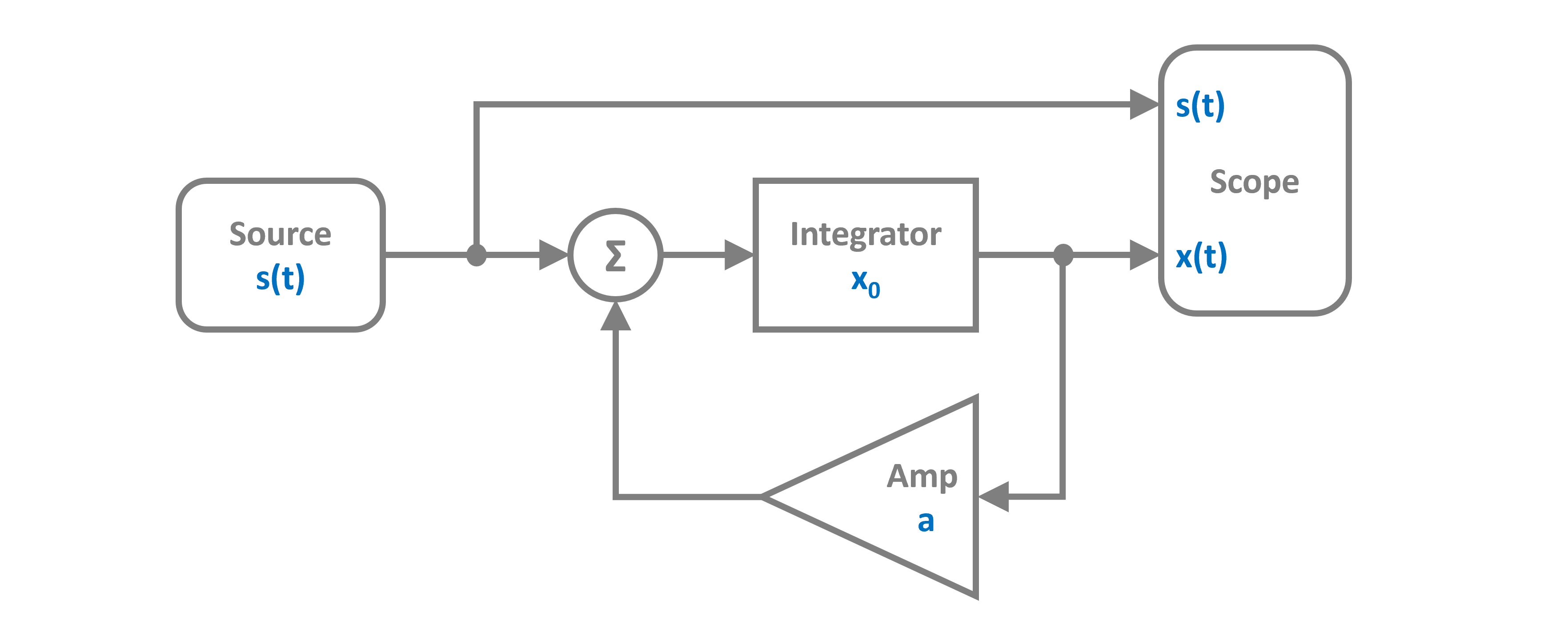
The block diagramm above can be translated to a netlist by using the blocks and the connection class provided by PathSim. First lets import the Simulation and Connection classes and the required blocks from the block library:

import matplotlib.pyplot as plt

# Apply PathSim docs matplotlib style for consistent, theme-friendly figures
plt.style.use('../pathsim_docs.mplstyle')

from pathsim import Simulation, Connection
from pathsim.blocks import Source, Integrator, Amplifier, Adder, Scope

Then lets define the system parameters such as the initial value x0 of the integrator, the linear feedback gain a and the time dependend source function s(t).

# System parameters
a, x0 = -1, 2

# Delay for step function
tau = 3

# Step function
def s(t):
    return int(t>tau)

Now we can construct the system by instantiating the blocks we need with their corresponding prameters and collect them together in a list:

# Blocks that define the system
Src = Source(s)
Int = Integrator(x0)
Amp = Amplifier(a)
Add = Adder()
Sco = Scope(labels=["step", "response"])

blocks = [Src, Int, Amp, Add, Sco]

Afterwards, the connections between the blocks can be defined. The first argument of the Connection class is the source block and its port (Src[0] would be port 0 of the instance of the Source block, which is also the default port).

# The connections between the blocks
connections = [
    Connection(Src, Add[0], Sco[0]),
    Connection(Amp, Add[1]),
    Connection(Add, Int),
    Connection(Int, Amp, Sco[1])
]

Finally we can instantiate the Simulation with the blocks, connections and some additional parameters such as the timestep. In this case, no special ODE solver is specified, so PathSim uses the default SSPRK22 integrator which is a fixed step 2nd order explicit Runge-Kutta method. A good starting point. Then we can run the simulation for some duration which is set as 4*tau in this example.

# Initialize simulation with the blocks, connections, timestep
Sim = Simulation(blocks, connections, dt=0.01, log=True)

# Run the simulation for some time
Sim.run(4*tau)

08:58:35 - INFO - LOGGING (log: True)
08:58:35 - INFO - BLOCKS (total: 5, dynamic: 1, static: 4, eventful: 0)
08:58:35 - INFO - GRAPH (nodes: 5, edges: 6, alg. depth: 3, loop depth: 0, runtime: 0.053ms)
08:58:35 - INFO - STARTING -> TRANSIENT (Duration: 12.00s)
08:58:35 - INFO - --------------------   1% | 0.0s<0.1s | 16106.6 it/s
08:58:35 - INFO - ####----------------  20% | 0.0s<0.1s | 17362.1 it/s
08:58:35 - INFO - ########------------  40% | 0.0s<0.0s | 17130.1 it/s
08:58:35 - INFO - ############--------  60% | 0.0s<0.0s | 17138.5 it/s
08:58:35 - INFO - ################----  80% | 0.1s<0.0s | 16462.1 it/s
08:58:35 - INFO - #################### 100% | 0.1s<--:-- | 17138.5 it/s
08:58:35 - INFO - FINISHED -> TRANSIENT (total steps: 1201, successful: 1201, runtime: 75.82 ms)

{'total_steps': 1201,
 'successful_steps': 1201,
 'runtime_ms': 75.82430000184104}

Due to the object oriented and decentralized nature of PathSim, the Scope block holds the recorded time series data from the simulation internally. It can be accessed by its read method

# Read the data from the scope
time, [data_step, data_response] = Sco.read()

or plotted directly in an external matplotlib window using the plot method

# Plot the results from the scope
fig, ax = Sco.plot()
plt.show()